jaccard

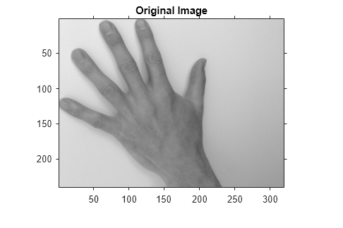
Read an image containing an object to segment. Convert the image to grayscale, and display the result.

A = imread('hands1.jpg');
I = im2gray(A);
figure
imshow(I)
title('Original Image')

Use the active contours (snakes) method to segment the hand.

mask = false(size(I));
mask(25:end-25,25:end-25) = true;
BW = activecontour(I, mask, 300);

Read in the ground truth against which to compare the segmentation.

BW_groundTruth = imread('hands1-mask.png');

Compute the Jaccard index of this segmentation.

similarity = jaccard(BW, BW_groundTruth);

Display the masks on top of each other. Colors indicate differences in the masks.

figure
imshowpair(BW, BW_groundTruth)
title(['Jaccard Index = ' num2str(similarity)])

This example shows how to segment an image into multiple regions. The example then computes the Jaccard similarity coefficient for each region.

Read in an image with several regions to segment.

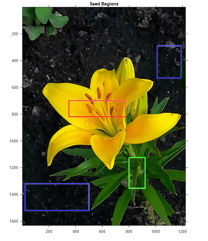
RGB = imread('yellowlily.jpg');

Create scribbles for three regions that distinguish their typical color characteristics. The first region classifies the yellow flower. The second region classifies the green stem and leaves. The last region classifies the brown dirt in two separate patches of the image. Regions are specified by a 4-element vector, whose elements indicate the x- and y-coordinate of the upper left corner of the ROI, the width of the ROI, and the height of the ROI.

region1 = [350 700 425 120]; % [x y w h] format
BW1 = false(size(RGB,1),size(RGB,2));
BW1(region1(2):region1(2)+region1(4),region1(1):region1(1)+region1(3)) = true;

region2 = [800 1124 120 230];
BW2 = false(size(RGB,1),size(RGB,2));
BW2(region2(2):region2(2)+region2(4),region2(1):region2(1)+region2(3)) = true;

region3 = [20 1320 480 200; 1010 290 180 240]; 
BW3 = false(size(RGB,1),size(RGB,2));    
BW3(region3(1,2):region3(1,2)+region3(1,4),region3(1,1):region3(1,1)+region3(1,3)) = true;
BW3(region3(2,2):region3(2,2)+region3(2,4),region3(2,1):region3(2,1)+region3(2,3)) = true;

Display the seed regions on top of the image.

figure
imshow(RGB)
hold on
visboundaries(BW1,'Color','r');
visboundaries(BW2,'Color','g');
visboundaries(BW3,'Color','b');
title('Seed Regions')

Segment the image into three regions using geodesic distance-based color segmentation.

L = imseggeodesic(RGB,BW1,BW2,BW3,'AdaptiveChannelWeighting',true);

Load a ground truth segmentation of the image.

L_groundTruth = double(imread('yellowlily-segmented.png'));

Visually compare the segmentation results with the ground truth.

figure
imshowpair(label2rgb(L),label2rgb(L_groundTruth),'montage')
title('Comparison of Segmentation Results (Left) and Ground Truth (Right)')

Compute the Jaccard similarity index (IoU) for each segmented region.

similarity = jaccard(L, L_groundTruth)

similarity = 3×1

    0.8861
    0.5683
    0.8414

The Jaccard similarity index is noticeably smaller for the second region. This result is consistent with the visual comparison of the segmentation results, which erroneously classifies the dirt in the lower right corner of the image as leaves.