Main Content

bfscore

Contour matching score for image segmentation

Description

score = bfscore(prediction,groundTruth) computes the BF (Boundary F1) contour matching score between the predicted segmentation in prediction and the true segmentation in groundTruth. prediction and groundTruth can be a pair of logical arrays for binary segmentation, or a pair of label or categorical arrays for multiclass segmentation.

example

[score,precision,recall] = bfscore(prediction,groundTruth) also returns the precision and recall values for the prediction image compared to the groundTruth image.

[___] = bfscore(prediction,groundTruth,threshold) computes the BF score using a specified threshold as the distance error tolerance, to decide whether a boundary point has a match or not.

Examples

collapse all

Read an image with an object to segment. Convert the image to grayscale, and display the result.

A = imread('hands1.jpg');
I = im2gray(A); 
figure
imshow(I)
title('Original Image')

Figure contains an axes object. The hidden axes object with title Original Image contains an object of type image.

Use the active contours (snakes) method to segment the hand.

mask = false(size(I));
mask(25:end-25,25:end-25) = true;
BW = activecontour(I, mask, 300);

Read the ground truth segmentation.

BW_groundTruth = imread('hands1-mask.png');

Compute the BF score of the active contours segmentation against the ground truth.

similarity = bfscore(BW, BW_groundTruth);

Display the masks on top of each other. Colors indicate differences in the masks.

figure
imshowpair(BW, BW_groundTruth)
title(['BF Score = ' num2str(similarity)])

Figure contains an axes object. The hidden axes object with title BF Score = 0.76266 contains an object of type image.

This example shows how to segment an image into multiple regions. The example then computes the BF score for each region.

Read an image with several regions to segment.

RGB = imread('yellowlily.jpg');

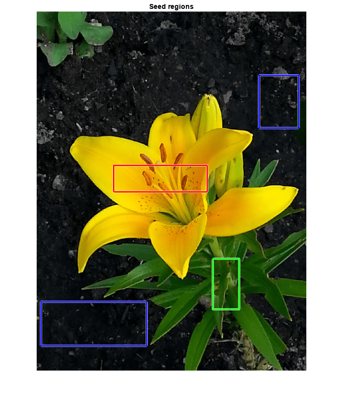
Create scribbles for three regions that distinguish their typical color characteristics. The first region classifies the yellow flower. The second region classifies the green stem and leaves. The last region classifies the brown dirt in two separate patches of the image. Regions are specified by a 4-element vector, whose elements indicate the x- and y-coordinate of the upper left corner of the ROI, the width of the ROI, and the height of the ROI.

region1 = [350 700 425 120]; % [x y w h] format
BW1 = false(size(RGB,1),size(RGB,2));
BW1(region1(2):region1(2)+region1(4),region1(1):region1(1)+region1(3)) = true;

region2 = [800 1124 120 230];
BW2 = false(size(RGB,1),size(RGB,2));
BW2(region2(2):region2(2)+region2(4),region2(1):region2(1)+region2(3)) = true;

region3 = [20 1320 480 200; 1010 290 180 240]; 
BW3 = false(size(RGB,1),size(RGB,2));    
BW3(region3(1,2):region3(1,2)+region3(1,4),region3(1,1):region3(1,1)+region3(1,3)) = true;
BW3(region3(2,2):region3(2,2)+region3(2,4),region3(2,1):region3(2,1)+region3(2,3)) = true;

Display the seed regions on top of the image.

figure
imshow(RGB)
hold on
visboundaries(BW1,'Color','r');
visboundaries(BW2,'Color','g');
visboundaries(BW3,'Color','b');
title('Seed regions')

Figure contains an axes object. The hidden axes object with title Seed regions contains 7 objects of type line, image.

Segment the image into three regions using geodesic distance-based color segmentation.

L = imseggeodesic(RGB,BW1,BW2,BW3,'AdaptiveChannelWeighting',true);

Load a ground truth segmentation of the image.

L_groundTruth = double(imread('yellowlily-segmented.png'));

Visually compare the segmentation results with the ground truth.

figure
imshowpair(label2rgb(L),label2rgb(L_groundTruth),'montage')
title('Comparison of Segmentation Results (Left) and Ground Truth (Right)')

Figure contains an axes object. The hidden axes object with title Comparison of Segmentation Results (Left) and Ground Truth (Right) contains an object of type image.

Compute the BF score for each segmented region.

similarity = bfscore(L, L_groundTruth)
similarity = 3×1

    0.7992
    0.5333
    0.7466

The BF score is noticeably smaller for the second region. This result is consistent with the visual comparison of the segmentation results, which erroneously classifies the dirt in the lower right corner of the image as leaves.

Input Arguments

collapse all

Predicted segmentation, specified as a 2-D or 3-D logical, numeric, or categorical array. If prediction is a numeric array, then it represents a label array and must contain nonnegative integers of data type double.

Data Types: logical | double | categorical

Ground truth segmentation, specified as a 2-D or 3-D logical, numeric, or categorical array of the same size and data type as prediction. If groundTruth is a numeric array, then it represents a label array and must contain nonnegative integers of data type double.

Data Types: logical | double | categorical

Distance error tolerance threshold in pixels, specified as a positive scalar. The threshold determines whether a boundary point has a match or not. If threshold is not specified, then the default value is 0.75% of the length of the image diagonal.

Example: 3

Data Types: double

Output Arguments

collapse all

BF score, returned as a numeric scalar or vector with values in the range [0, 1]. A score of 1 means that the contours of objects in the corresponding class in prediction and groundTruth are a perfect match. If the input arrays are:

  • logical arrays, score is a scalar and represents the BF score of the foreground.

  • label or categorical arrays, score is a vector. The first coefficient in score is the BF score for the first foreground class, the second coefficient is the score for the second foreground class, and so on.

Precision, returned as a numeric scalar or numeric vector with values in the range [0, 1]. Each element indicates the precision of object contours in the corresponding foreground class.

Precision is the ratio of the number of points on the boundary of the predicted segmentation that are close enough to the boundary of the ground truth segmentation to the length of the predicted boundary. In other words, precision is the fraction of detections that are true positives rather than false positives.

Recall, returned as a numeric scalar or numeric vector with values in the range [0, 1]. Each element indicates the recall of object contours in the corresponding foreground class.

Recall is the ratio of the number of points on the boundary of the ground truth segmentation that are close enough to the boundary of the predicted segmentation to the length of the ground truth boundary. In other words, recall is the fraction of true positives that are detected rather than missed.

More About

collapse all

BF (Boundary F1) Score

The BF score measures how close the predicted boundary of an object matches the ground truth boundary.

The BF score is defined as the harmonic mean (F1-measure) of the precision and recall values with a distance error tolerance to decide whether a point on the predicted boundary has a match on the ground truth boundary or not.

score = 2 * precision * recall / (recall + precision)

References

[1] Csurka, G., D. Larlus, and F. Perronnin. "What is a good evaluation measure for semantic segmentation?" Proceedings of the British Machine Vision Conference, 2013, pp. 32.1-32.11.

Extended Capabilities

Version History

Introduced in R2017b

expand all

See Also

|