Target Detection Using Spectral Signature Matching

Read Test Data

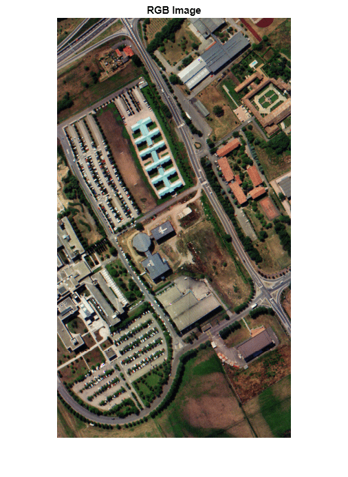
Read the test data from Pavia University dataset by using the hypercube function. The function returns a hypercube object that stores the data cube and the metadata information read from the test data. The test data has 103 spectral bands and their wavelengths range from 430 nm to 860 nm. The geometric resolution is 1.3 meters and the spatial resolution of each band image is 610-by-340.

hcube = hypercube("paviaU.hdr");

Estimate an RGB color image from the data cube by using the colorize function. Set the ContrastStretching parameter value to true in order to improve the contrast of RGB color image. Display the RGB image.

rgbImg = colorize(hcube,Method="rgb",ContrastStretching=true);
imshow(rgbImg)
title("RGB Image")

Read Reference Spectrum

Read the spectral information corresponding to a roofing material from the ECOSTRESS spectral library by using the readEcostressSig function.

lib = readEcostressSig("manmade.roofingmaterial.metal.solid.all.0692uuucop.jhu.becknic.spectrum.txt");

Inspect the properties of the reference spectrum read from the ECOSTRESS library. The output structure lib stores the metadata and the data values read from the ECOSTRESS library.

lib

lib = struct with fields:
                     Name: "Copper Metal"
                     Type: "manmade"
                    Class: "Roofing Material"
                 SubClass: "Metal"
             ParticleSize: "Solid"
                    Genus: [0x0 string]
                  Species: [0x0 string]
                 SampleNo: "0692UUUCOP"
                    Owner: "National Photographic Interpretation Center"
          WavelengthRange: "All"
                   Origin: "Spectra obtained from the Noncoventional Exploitation FactorsData System of the National Photographic Interpretation Center."
           CollectionDate: "N/A"
              Description: "Extremely weathered bare copper metal from government building roof flashing. Original ASTER Spectral Library name was jhu.becknic.manmade.roofing.metal.solid.0692uuu.spectrum.txt"
              Measurement: "Directional (10 Degree) Hemispherical Reflectance"
              FirstColumn: "X"
             SecondColumn: "Y"
           WavelengthUnit: "micrometer"
                 DataUnit: "Reflectance (percent)"
              FirstXValue: "0.3000"
               LastXValue: "12.5000"
          NumberOfXValues: "536"
    AdditionalInformation: "none"
               Wavelength: [536x1 double]
              Reflectance: [536x1 double]

Read the wavelength and the reflectance values stored in lib. The wavelength and the reflectance pair comprises the reference spectrum or the reference spectral signature.

wavelength = lib.Wavelength;
reflectance = lib.Reflectance;

Plot the reference spectrum read from the ECOSTRESS library.

plot(wavelength,reflectance,LineWidth=2)
axis tight
xlabel("Wavelength (\mum)")
ylabel("Reflectance (%)")
title("Reference Spectrum")

Perform Spectral Matching

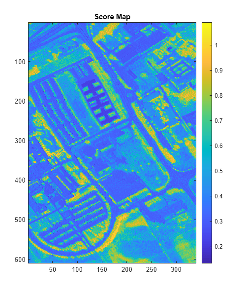
Find the spectral similarity between the reference spectrum and the data cube by using the spectralMatch function. By default, the function uses the spectral angle mapper (SAM) method for finding the spectral match. The output is a score map that signifies the matching between each pixel spectrum and the reference spectrum. Thus, the score map is a matrix of spatial dimension same as that of the test data. In this case, the size of the score map is 610-by-340. SAM is insensitive to gain factors and hence, can be used to match pixel spectrum that inherently have an unknown gain factor due to topographic illumination effects.

scoreMap = spectralMatch(lib,hcube);

Display the score map.

figure(Position=[0 0 500 600])
imagesc(scoreMap)
colormap parula
colorbar
title("Score Map")

Classify and Detect Target

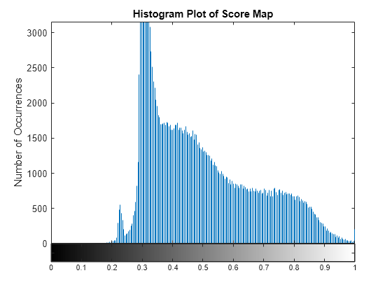
Typical values for the SAM score lie in the range [0, 3.142] and the measurement unit is radians. A lower value of the SAM score represents better matching between the pixel spectrum and the reference spectrum. Use a thresholding approach to spatially localize the target region in the input data. To determine the threshold, inspect the histogram of the score map. The minimum SAM score value with prominent number of occurrences can be used to select the threshold for detecting the target region.

figure
imhist(scoreMap);
title("Histogram Plot of Score Map")
xlabel("Score Map Values")
ylabel("Number of Occurrences")

From the histogram plot, you can infer the minimum score value with prominent number of occurrence as approximately 0.22. Accordingly, you can set a value around the local maxima as the threshold. For this example, you can select the threshold for detecting the target as 0.25. The pixel values that are less than the maximum threshold are classified as the target region.

maxthreshold = 0.25;

Perform thresholding to detect the target region with maximum spectral similarity. Overlay the thresholded image on the RGB image of the hyperspectral data.

thresholdedImg = scoreMap <= maxthreshold;
overlaidImg = imoverlay(rgbImg,thresholdedImg,"green");

Display the results.

fig = figure(Position=[0 0 900 500]);
axes1 = axes(Parent=fig,Position=[0.04 0.11 0.4 0.82]);
imagesc(thresholdedImg,Parent=axes1);
colormap([0 0 0;1 1 1])
title("Detected Target Region")
axis off
axes2 = axes(Parent=fig,Position=[0.47 0.11 0.4 0.82]);
imagesc(overlaidImg,Parent=axes2)
axis off
title("Overlaid Detection Results")

Validate Detection Results

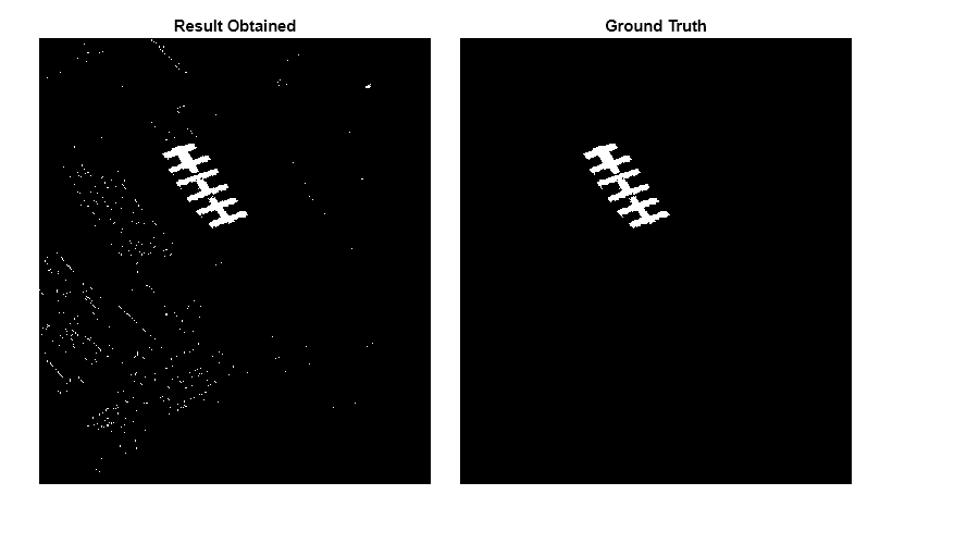
You can validate the obtained target detection results by using the ground truth data taken from Pavia University dataset.

Load a MAT file containing the ground truth data. To validate the result quantitatively, calculate the mean squared error between the ground truth and the output. The error value is less if the obtained results are close to the ground truth.

load("paviauRoofingGT.mat");
err = immse(im2double(paviauRoofingGT), im2double(thresholdedImg));
disp("The mean squared error is "+err)

The mean squared error is 0.004026

fig = figure(Position=[0 0 900 500]);
axes1 = axes(Parent=fig,Position=[0.04 0.11 0.4 0.82]);
imagesc(thresholdedImg,Parent=axes1);
colormap([0 0 0;1 1 1]);
title("Result Obtained")
axis off
axes2 = axes(Parent=fig,Position=[0.47 0.11 0.4 0.82]);
imagesc(paviauRoofingGT,Parent=axes2)
colormap([0 0 0;1 1 1]);
axis off
title("Ground Truth")

References

[1] Kruse, F.A., A.B. Lefkoff, J.W. Boardman, K.B. Heidebrecht, A.T. Shapiro, P.J. Barloon, and A.F.H. Goetz. “The Spectral Image Processing System (SIPS)—Interactive Visualization and Analysis of Imaging Spectrometer Data.” Remote Sensing of Environment 44, no. 2–3 (May 1993): 145–63. https://doi.org/10.1016/0034-4257(93)90013-N.

[2] Chein-I Chang. “An Information-Theoretic Approach to Spectral Variability, Similarity, and Discrimination for Hyperspectral Image Analysis.” IEEE Transactions on Information Theory 46, no. 5 (August 2000): 1927–32. https://doi.org/10.1109/18.857802.

[3] ECOSTRESS Spectral Library: https://speclib.jpl.nasa.gov

[4] Meerdink, Susan K., Simon J. Hook, Dar A. Roberts, and Elsa A. Abbott. “The ECOSTRESS Spectral Library Version 1.0.” Remote Sensing of Environment 230 (September 2019): 111196. https://doi.org/10.1016/j.rse.2019.05.015.

[5] Baldridge, A.M., S.J. Hook, C.I. Grove, and G. Rivera. “The ASTER Spectral Library Version 2.0.” Remote Sensing of Environment 113, no. 4 (April 2009): 711–15. https://doi.org/10.1016/j.rse.2008.11.007.