pcheatmap
Syntax
Description
ax = pcheatmap(ptCloudA,ptCloudB,mapData)mapData. The
function displays the point clouds using color information, if available. Otherwise, the
function uses dark gray and light gray to display ptCloudA and
ptCloudB, respectively. The function returns an axes graphics
object.
ax = pcheatmap(___,Name=Value)MarkerSize=5 sets
the diameter of the point marker to 5.
Examples
Read two point clouds into the workspace.
load("aerialLidarData")
referencePointCloud = aerialLidarData{1};
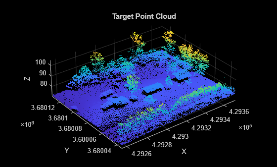
targetPointCloud = aerialLidarData{2};Visualize both point clouds. Notice that the target point cloud includes an additional house that is missing from the reference point cloud.
figure
pcshow(referencePointCloud)
xlabel("X")
ylabel("Y")
zlabel("Z")
title("Reference Point Cloud")

figure
pcshow(targetPointCloud)
xlabel("X")
ylabel("Y")
zlabel("Z")
title("Target Point Cloud")
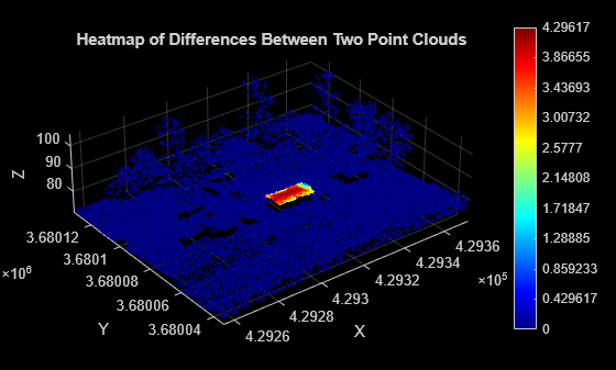
Compute the distance between the two point clouds.
dists = pcdistance(targetPointCloud,referencePointCloud);
Visualize the differences between the two point clouds as a heatmap. Notice that the heatmap highlights the change, an additional house in the target point cloud.
figure
pcheatmap(targetPointCloud,dists)
xlabel("X")
ylabel("Y")
zlabel("Z")
title("Heatmap of Differences Between Two Point Clouds")
Input Arguments
Name-Value Arguments
Specify optional pairs of arguments as
Name1=Value1,...,NameN=ValueN, where Name is
the argument name and Value is the corresponding value.
Name-value arguments must appear after other arguments, but the order of the
pairs does not matter.
Example: pcheatmap(ptCloudA,mapData,MarkerSize=5) sets the diameter of
the point marker to 5.
Colormap, specified as an N-by-3 numeric matrix with values in the range [0, 1]. Each row is a three-element RGB triplet that specifies the red, green, and blue components of a single color of the colormap.
Note
Changing the colormap of the figure or axes does not affect the heatmap colors.
Data Types: single | double
Colormap range for the map data mapData, specified as a
two-element vector. The default value is [min(mapData(:))
max(mapData(:))]. If the map data contains values below the minimum or
above the maximum of this range, the function maps those values to the first or the
last color in the colormap, respectively. The function maps intermediate values
linearly to the corresponding colors in the colormap.
Data Types: single | double | int8 | int16 | int32 | int64 | uint8 | uint16 | uint32 | uint64
Diameter of the marker, specified as a positive scalar. This value specifies the approximate diameter of the point marker. MATLAB® graphics defines the unit as points. A marker size larger than 6 can reduce rendering performance.
Data Types: single | double | int8 | int16 | int32 | int64 | uint8 | uint16 | uint32 | uint64
Background color, specified as an RGB triplet, hexadecimal color code, or a long or short color name.
This table lists the named color options, the equivalent RGB triplets, and the hexadecimal color codes.
| Color Name | Short Name | RGB Triplet | Hexadecimal Color Code | Appearance |
|---|---|---|---|---|
"red" | "r" | [1 0 0] | "#FF0000" |
|
"green" | "g" | [0 1 0] | "#00FF00" |
|
"blue" | "b" | [0 0 1] | "#0000FF" |
|
"cyan"
| "c" | [0 1 1] | "#00FFFF" |
|
"magenta" | "m" | [1 0 1] | "#FF00FF" |
|
"yellow" | "y" | [1 1 0] | "#FFFF00" |
|
"black" | "k" | [0 0 0] | "#000000" |
|
"white" | "w" | [1 1 1] | "#FFFFFF" |
|
Data Types: char | string | uint8 | uint16 | int16 | double | single
Vertical axis, specified as "X", "Y", or
"Z". This value sets the selected axis of the point cloud as the
vertical axis.
Vertical axis direction, specified as "Up" or
"Down".
Camera projection for 3-D views, specified as one of these values:
"perspective"— Projects the viewing volume as the frustum of a pyramid (a pyramid whose apex has been cut off parallel to the base). Objects further from the camera appear smaller. Distance causes foreshortening, which enables you to perceive the depth of 3-D objects. This projection type is useful when you want to display realistic views of real objects. Perspective projection does not preserve the relative dimensions of objects. Instead, it displays a distant line segment smaller than a nearer line segment of the same length. Lines that are parallel in the data might not appear parallel in the scene."orthographic"— This projection type maintains the correct relative dimensions of graphics objects regarding the distance of a given point from the viewer. Relative distance from the camera does not affect the size of objects. Lines that are parallel in the data appear parallel on the screen. This projection type is useful when it is important to maintain the actual size of objects and the angles between objects.
Plane on which to visualize the point cloud, specified as
"auto", "XY", "YX",
"XZ", "ZX", "YZ", or
"ZY". The ViewPlane argument sets the line
of sight from the camera, centered in the selected plane, to the center of the
plot.
State of axes visibility, specified as "on" or
"off", or as numeric or logical 0
(false) or 1 (true). A
value of "on" is equivalent to true, and
"off" is equivalent to false. Thus, you can
use the value of this property as a logical value. The value is stored as an on/off
logical value of type matlab.lang.OnOffSwitchState.
"on"— Display the axes and its children."off"— Hide the axes without deleting it. You can still access the properties of an invisible axes object. Note that child objects such as lines remain visible.
Data Types: logical
Axes on which to display the visualization, specified as an Axes
object. To create an Axes object, use the axes function. To display the visualization in a new figure, leave
Parent unspecified.
Output Arguments
Version History
Introduced in R2026a