Create Map Displays with Geographic Data
Many geospatial data sets contain geographic data, which is data referenced to latitude and longitude coordinates. This example shows how to import geographic data, display the data on an axesm-based map, and customize the map. Within the example:
Import vector and raster data files that contain geographic data.
Create maps. Visualize vector data, raster data, and a mixture of vector and raster data on the maps.
Customize a map by adding a scale ruler, a north arrow, and an inset map.
This example creates map displays using axesm-based maps. For information about other 2-D map display options, see Choose a 2-D Map Display.
Import Points, Lines, and Polygons in Geographic Coordinates
A variety of data formats can store geographic vector data, including the shapefile and GPX formats. Use the readgeotable function to read vector data into the workspace as a geospatial table.
usastatehi.shpis a shapefile that contains US states. The file represents the states using polygon shapes in geographic coordinates.boston_placenames.gpxis a GPX file that contains places in Boston, MA. The file represents the places using point shapes in geographic coordinates.sample_route.gpxis a GPX file that contains a GPS route from Boston, MA to Natick, MA. The file represents the route using a line shape in geographic coordinates.
states = readgeotable("usastatehi.shp");
places = readgeotable("boston_placenames.gpx");
route = readgeotable("sample_route.gpx",Layer="routes");
Display Polygons in Geographic Coordinates
Display the shapes on an axesm-based map (previously referred to as map axes). axesm-based maps are useful for plotting geographic data in a mixture of vector and raster formats. For more information about other map display options, see Choose a 2-D Map Display.
The extent of the data is in the United States, so set up the map by using the usamap function. Then, project and display the shapes on the map by using the geoshow function. Change the background of the map to an ocean color by setting the face color of the map frame.
figure
ax = usamap("conus");
geoshow(states)
oceanColor = [0.3010 0.7450 0.9330];
setm(ax,"FFaceColor",oceanColor)
Add a title.
title("Conterminous US States")
Display Points and Lines in Geographic Coordinates
Extract the polygon shape for Massachusetts from the geospatial table of US states.
ma = geocode("Massachusetts",states);Set up a new axesm-based map for a region surrounding Massachusetts. Change the background of the map to an ocean color. Provide geographic context for the map by displaying the US states in one color and Massachusetts in a second color.
figure
ax = usamap("Massachusetts");
setm(ax,"FFaceColor",oceanColor)
geoshow(states)
maColor = [0.4660 0.6740 0.1880];
geoshow(ma,FaceColor=maColor)
Display the places and the route on the same map.
geoshow(places)
geoshow(route)
Add a title and a subtitle.
title("Massachusetts and Surrounding Region")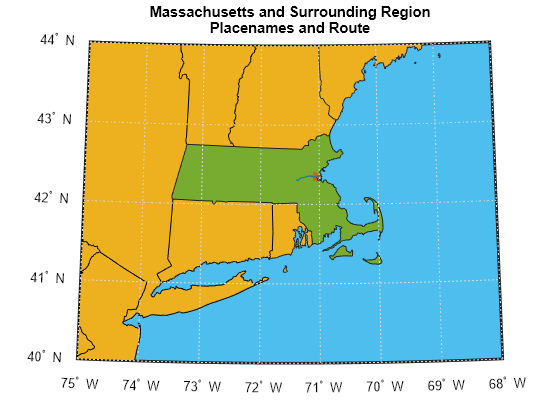
Specify Latitude and Longitude Limits of Map
Create two areas of interest (AOIs) from the places and route. Buffer the AOIs by 0.05 degrees. Then, calculate the latitude and longitude limits of the buffered AOIs.
aoiPlaces = aoiquad(places);
aoiRoute = aoiquad(route);
buffered = buffer([aoiRoute aoiPlaces],0.05);
[latlim,lonlim] = bounds(buffered,"all");
Create a new axesm-based map using the new limits.
figure
ax = usamap(latlim,lonlim);
setm(ax,"FFaceColor",oceanColor)
Display the Massachusetts shape, the places, and the route on the new map.
geoshow(ma,FaceColor=maColor)
geoshow(places)
geoshow(route)
Add a title.
title("Closeup of Places and Route")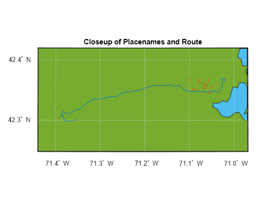
Import Raster Data in Geographic Coordinates
A variety of data formats can store geographic raster data.
To read raster data in formats such as GeoTIFF, Esri Grid, DTED, and ENVI, use the
readgeorasterfunction.To read an image associated with a worldfile, use the
imreadandworldfilereadfunctions. Theimreadfunction reads the image, and theworldfilereadfunction uses the worldfile to create a raster reference object.
Import an overview image for a region surrounding Boston, Massachusetts. The coordinates of the overview image are in geographic coordinates.
filename = "boston_ovr.jpg";
worldfilename = getworldfilename(filename);

RGB = imread(filename);
R = worldfileread(worldfilename,"geographic",size(RGB));
Display Raster Data in Geographic Coordinates
Create a new axesm-based map from the overview image and the raster reference object. The limits of the map match the limits stored in the reference object. Customize the map by specifying the locations of the meridian and parallel labels, and by specifying the number of decimal places to include in the labels.
figure
ax = usamap(RGB,R);
setm(ax,"MLabelLocation",0.05,"PLabelLocation",0.05,"MLabelRound",-2,"PLabelRound",-2)
Display the image on the map. Add a title.
geoshow(RGB,R)
title("Boston Overview")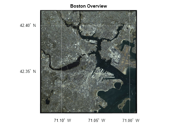
Display Vector and Raster Data on Same Map
Get new latitude and longitude limits from the places, the route, and the image. Create a new axesm-based map that uses the new latitude and longitude limits.
aoiImage = aoiquad(R);
[latlim,lonlim] = bounds([aoiPlaces aoiRoute aoiImage],"all");

figure
ax = usamap(latlim,lonlim);
setm(ax,"GColor","k","PLabelLocation",0.05,"PLineLocation",0.05)
Display the image, the outline of Massachusetts, the places, and the route on the new map.
geoshow(RGB,R)
geoshow(ma,FaceColor="none",EdgeColor="y",LineWidth=2)
geoshow(places)
geoshow(route)
Add a title.
title("Boston Overview and Geographic Vector Data")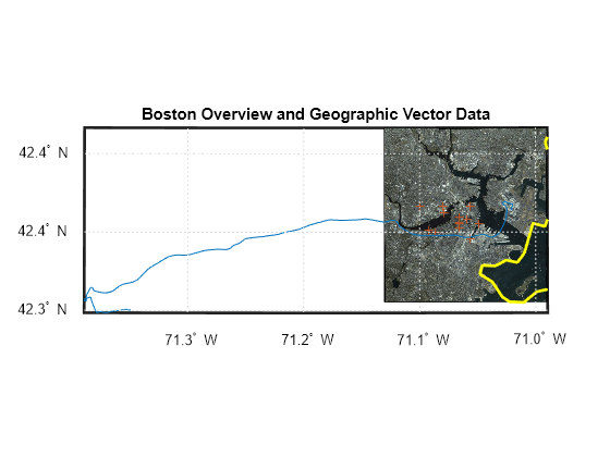
Customize Map
Customize a map by adding a scale ruler, a north arrow, and an inset map.
Add Scale Ruler
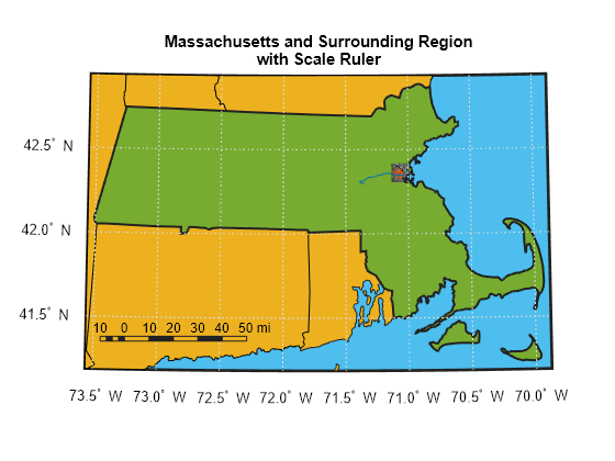
Customize a map display by including a scale ruler. A scale ruler is a graphic object that shows distances on the ground at the correct size for the projection. This example shows how to create a scale ruler that displays horizontal distances in international miles.
Buffer the Massachusetts shape by 0.05 degrees. Then, find the limits of the buffered shape.
bufferedMA = buffer(ma.Shape,0.05);
[latlim,lonlim] = bounds(bufferedMA);
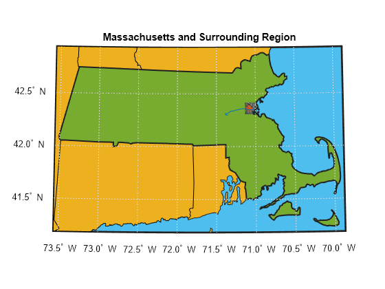
Create a new map that contains the US states, Massachusetts, the overview image, the places, and the route. Add a title.
figure
ax = usamap(latlim,lonlim);
setm(ax,"FFaceColor",oceanColor)
geoshow(states)
geoshow(ma,FaceColor=maColor)
geoshow(RGB,R)
geoshow(places)
geoshow(route)
title("Massachusetts and Surrounding Region")
Specify a location for the scale ruler. You can interactively determine a location for the scale ruler by using the ginput function: [xLoc,yLoc] = ginput(1);
Alternatively, use a predetermined location.
xLoc = -127800;
yLoc = 5014700;
Add a scale ruler to the map.
scaleruler(Units="mi",RulerStyle="patches",XLoc=xLoc,YLoc=yLoc)
Add North Arrow
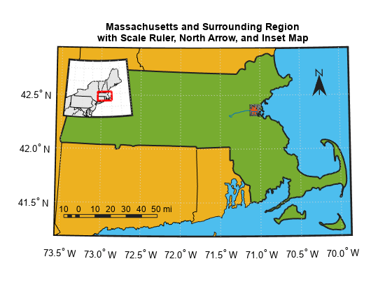
Customize the map by adding a north arrow. A north arrow is a graphic element that points to the geographic North Pole.
Specify latitude and longitude coordinates for the north arrow. Then, add the north arrow to the map.
northArrowLat =  42.5;
northArrowLon = -70.25;
northarrow(latitude=northArrowLat,Longitude=northArrowLon)

Add Inset Map
Customize the map by adding an inset map. An inset map is a smaller map displayed inside a larger map. You can use an inset map to create geographic context for the larger map. To create an inset map:
Create an axes object in the upper-left of the map frame.
Place a map inside the axes object. Customize the map by removing the parallel and meridian labels, setting the background color, and removing the grid lines.
Display the US states for the surrounding region.
Show the extent of the larger map using a red box.
h2 = axes(Position=[0.15 0.65 0.2 0.2],Visible="off");

usamap(["PA","ME"])
plabel off
mlabel off
gridm off
setm(h2,"FFaceColor","w")

geoshow(states,FaceColor=[0.9 0.9 0.9],Parent=h2)

mapAOI = aoiquad(latlim,lonlim);
T = table(mapAOI,VariableName="Shape");
geoshow(T,FaceColor="none",EdgeColor="r",LineWidth=2)
See Also
Functions
usamap|geoshow|scaleruler|northarrow