Experiment with Predator-Prey Equations

Since R2023b

This example shows how to use Experiment Manager to explore how different coefficient values and initial values affect the solution of a system of differential equations.

The Lotka-Volterra predator-prey model is a system of first-order ordinary differential equations that describes the relationship between two competing populations. For example, these equations describe the populations of rabbits and foxes with respect to time:

$R^{'} = (1 - \frac{F}{α}) R$

$F^{'} = - (1 - \frac{R}{β}) F$

In these equations, $R$ is the number of rabbits and $F$ is the number of foxes. The coefficients $α$ and $β$ describe the predation of rabbits by foxes. The population of rabbits increases when $F < α$ and decreases when $F > α$ . The population of foxes increases when $R > β$ and decreases when $R < β$ . For more information, see [1].

In this experiment, you observe the effect on the predicted populations of rabbits and foxes when you use different values for the coefficients $α$ and $β$ and the initial values of $R$ and $F$ .

Open Experiment

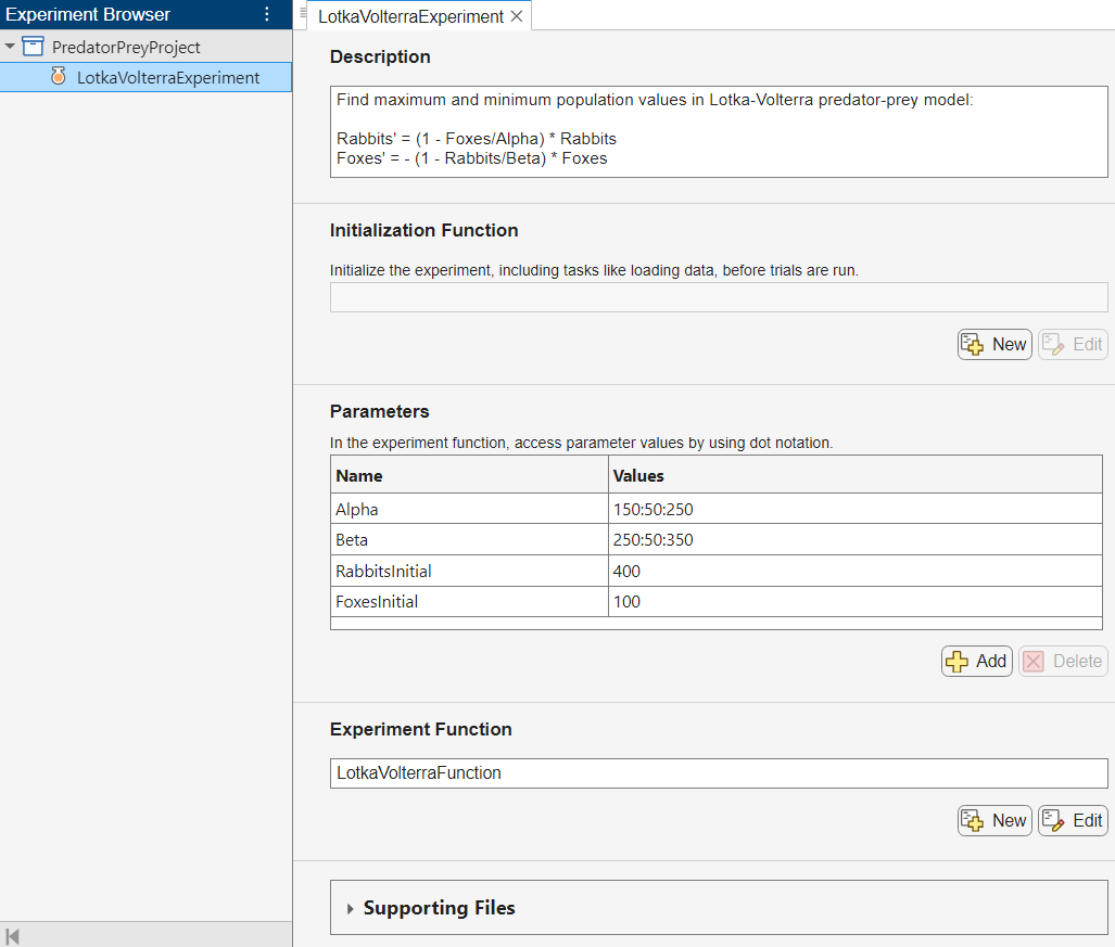
First, open the example. Experiment Manager loads a project with a preconfigured experiment that you can inspect and run. To open the experiment, in the Experiment Browser pane, double-click LotkaVolterraExperiment.

Experiment editor containing the experiment description, parameter names and values, and experiment function name

The experiment consists of a description, a table of parameters, and an experiment function.

The Description field contains a textual description of the experiment. For this example, the description is:

Find maximum and minimum population values in Lotka-Volterra predator-prey model:

Rabbits' = (1 - Foxes/Alpha) * Rabbits
Foxes' = -(1 - Rabbits/Beta) * Foxes

The Parameters section specifies the parameter values to use for the experiment. Experiment Manager runs multiple trials of your experiment using a different combination of parameters for each trial. This example uses the parameters Alpha and Beta to specify the values of the coefficients of the Lotka-Volterra equations and the parameters RabbitsInitial and FoxesInitial to specify the initial population of rabbits and foxes.

The Experiment Function section specifies the function LotkaVolterraFunction, which defines the procedure for the experiment. To open this function in MATLAB® Editor, click Edit. The code for the function also appears in Experiment Function. The input to the experiment function is a structure called params with fields from the parameter table. The function uses dot notation to extract the parameter values from this structure and to set up the initial conditions and differential equations for the predator-prey problem.

yInitial = [params.RabbitsInitial params.FoxesInitial]';
tRange = [0 20];
 
signs = [1 -1]';
mu = [params.Alpha params.Beta]';
dydt = @(t,y) signs.*(1-flipud(y)./mu).*y;

Next, the experiment function calls ode45 to solve the differential equations and to compute the maximum and minimum number of predicted rabbits and foxes.

[t,y] = ode45(dydt,tRange,yInitial);
 
RabbitsMin = min(y(:,1));
RabbitsMax = max(y(:,1));
FoxesMin = min(y(:,2));
FoxesMax = max(y(:,2));

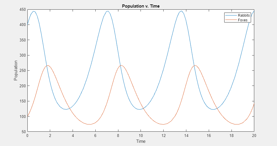
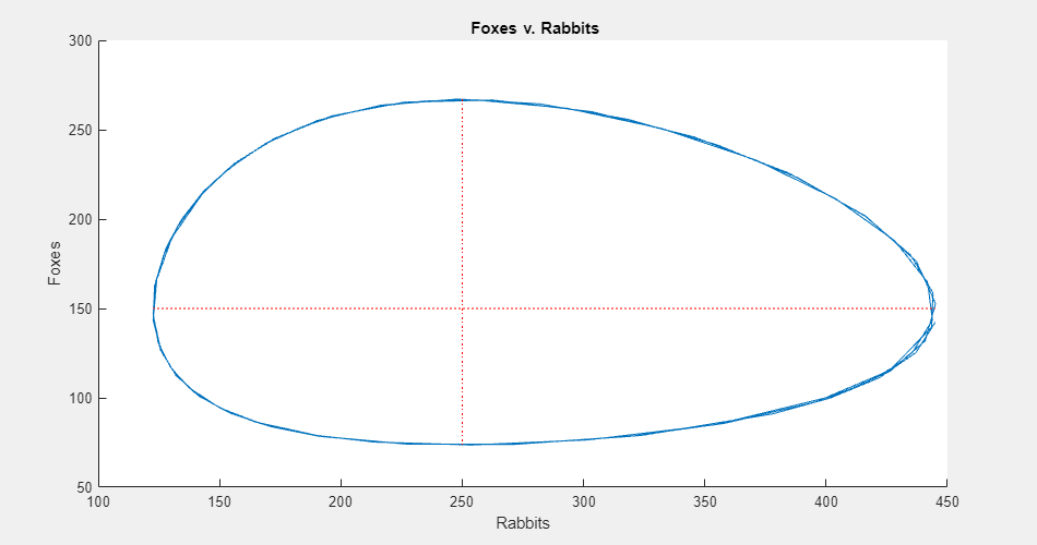
Finally, the experiment function plots the populations of rabbits and foxes against time and against each other. When you run the experiment, Experiment Manager adds two buttons to the Review Results gallery in the toolstrip so you can display these figures. The Name property of each figure specifies the name of the corresponding button in the toolstrip.

figure(Name="Population Size");
plot(t,y)
title("Population v. Time")
xlabel("Time")
ylabel("Population")
legend("Rabbits","Foxes")
 
figure(Name="Phase Plane");
hold on
plot(y(:,1),y(:,2))
plot([mu(2),mu(2)],[FoxesMin,FoxesMax],":r");
plot([RabbitsMin,RabbitsMax],[mu(1),mu(1)],":r");
title("Foxes v. Rabbits")
xlabel("Rabbits")
ylabel("Foxes")
hold off

Run Experiment

On the Experiment Manager toolstrip, click Run. Experiment Manager runs the experiment function nine times, each time using a different combination of parameter values. A table of results displays the output values for each trial.

Table of results containing columns for the experiment details, parameters, and outputs

Evaluate Results

To investigate how changing a parameter value affects the predicted populations of rabbits and foxes, you can sort the results table using one of the output values. For example, to find the trial with the largest rabbit population:

Point to the header of the RabbitsMax column.
Click the triangle icon.
Select Sort in Descending Order.

Table of results, where the RabbitsMax column is sorted in descending order

You can also select a trial in the results table and inspect the visualizations created by the experiment function. To see the predicted populations plotted as functions of time, on the Experiment Manager toolstrip, under Review Results, click Population Size. This plot shows the two populations oscillating, with the maximum and minimum values in the rabbit population preceding the maximum and minimum values in the fox population.

Population size versus time plot

To see the populations plotted against each other, click Phase Plane. The phase plane plot shows the cyclic relationship between the populations.

Fox population versus rabbit population phase plot

To perform additional computations on your results, you can export the results table to the MATLAB workspace as a nested table array. For example, to compare the peak-to-peak amplitudes of the populations over all the trials in your experiment:

On the Experiment Manager toolstrip, click Export.
In the dialog window, enter the name of a workspace variable for the exported table. The default name is resultsTable.
In the MATLAB Command Window, use the exported table as the input to the function populationAmplitudes:

populationAmplitudes(resultsTable)

To view the code for this function, see Compare Population Amplitudes. The function displays a summary of the maximum, minimum, and mean peak-to-peak population amplitudes for rabbits and foxes over all the trials in your experiment.

******************************************

Population of rabbits:
Maximum amplitude: 575.5 (Trial 9)
Minimum amplitude: 284.1 (Trial 7)
Mean amplitude: 416.9

Population of foxes:
Maximum amplitude: 473.9 (Trial 3)
Minimum amplitude: 121.2 (Trial 7)
Mean amplitude: 293.6

******************************************

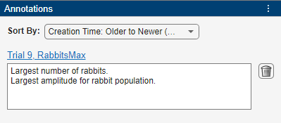
To record observations about the results of your experiment, add an annotation:

In the results table, right-click the RabbitsMax cell for trial 9.
Select Add Annotation.
In the Annotations pane, enter your observations in the text box.

Annotation for the cell in the table of results corresponding to Trial 9 and the RabbitsMax output: "Largest number of rabbits. Largest amplitude for rabbit population."

Experiment Function

This function solves the Lotka-Volterra equations, plots the predicted populations of rabbits and foxes over time and against each other, and returns the maximum and minimum number of rabbits and foxes. The input argument params is a structure with fields from the parameter table.

function [RabbitsMin,RabbitsMax,FoxesMin,FoxesMax] = LotkaVolterraFunction(params)

yInitial = [params.RabbitsInitial params.FoxesInitial]';
tRange = [0 20];
 
signs = [1 -1]';
mu = [params.Alpha params.Beta]';
dydt = @(t,y) signs.*(1-flipud(y)./mu).*y;
 
[t,y] = ode45(dydt,tRange,yInitial);
 
RabbitsMin = min(y(:,1));
RabbitsMax = max(y(:,1));
FoxesMin = min(y(:,2));
FoxesMax = max(y(:,2));
 
figure(Name="Population Size");
plot(t,y)
title("Population v. Time")
xlabel("Time")
ylabel("Population")
legend("Rabbits","Foxes")
 
figure(Name="Phase Plane");
hold on
plot(y(:,1),y(:,2))
plot([mu(2),mu(2)],[FoxesMin,FoxesMax],":r");
plot([RabbitsMin,RabbitsMax],[mu(1),mu(1)],":r");
title("Foxes v. Rabbits")
xlabel("Rabbits")
ylabel("Foxes")
hold off
 
end

Compute Population Amplitudes

This function extracts the maximum and minimum number of rabbits and foxes for each trial from the exported results table results. Then, the function computes the maximum, minimum, and mean peak-to-peak population amplitudes over all trials.

function populationAmplitudes(results)

results = splitvars(results);
RabbitsAmplitude = results.RabbitsMax - results.RabbitsMin;
FoxesAmplitude = results.FoxesMax - results.FoxesMin;
 
[maxRabbitsAmplitude,maxRabbitsAmplitudeTrial] = max(RabbitsAmplitude);
[minRabbitsAmplitude,minRabbitsAmplitudgeTrial] = min(RabbitsAmplitude);
meanRabbitsAmplitude = mean(RabbitsAmplitude);
 
[maxFoxesAmplitude,maxFoxesAmplitudeTrial] = max(FoxesAmplitude);
[minFoxesAmplitude,minFoxesAmplitudeTrial] = min(FoxesAmplitude);
meanFoxesAmplitude = mean(FoxesAmplitude);
 
fprintf("\n******************************************\n\n");
fprintf("Population of rabbits:\n");
fprintf("Maximum amplitude: %.1f (Trial %d)\n", ...
    maxRabbitsAmplitude,maxRabbitsAmplitudeTrial);
fprintf("Minimum amplitude: %.1f (Trial %d)\n", ...
    minRabbitsAmplitude,minRabbitsAmplitudgeTrial);
fprintf("Mean amplitude: %.1f \n\n",meanRabbitsAmplitude);
fprintf("Population of foxes:\n");
fprintf("Maximum amplitude: %.1f (Trial %d)\n", ...
    maxFoxesAmplitude,maxFoxesAmplitudeTrial);
fprintf("Minimum amplitude: %.1f (Trial %d)\n", ...
    minFoxesAmplitude,minFoxesAmplitudeTrial);
fprintf("Mean amplitude: %.1f \n",meanFoxesAmplitude);
fprintf("\n******************************************\n\n");
 
end

References

[1] Moler, Cleve. "Predator-Prey Model." In Experiments with MATLAB^®. Natick, MA: The MathWorks^®, 2011. mathworks.com/moler/exm.html.

Experiment with Predator-Prey Equations

Open Experiment

Run Experiment

Evaluate Results

Experiment Function

Compute Population Amplitudes

References

See Also

Apps

Functions

Related Topics