求解捕食者-猎物方程
此示例说明如何使用变步长龙格-库塔积分方法求解表示捕食者/猎物模型的微分方程。ode23 方法使用一对 2 阶和 3 阶公式实现中等精度,ode45 方法使用一对 4 阶和 5 阶公式实现更高的精度。
以名为 Lotka-Volterra 方程,也即捕食者-猎物模型的一对一阶常微分方程为例:
变量 和 分别计算猎物和捕食者的数量。二次交叉项表示品种之间的交叉。当没有捕食者时,猎物数量将增加,当猎物匮乏时,捕食者数量将减少。
编写方程代码
为了模拟系统,需要创建一个函数,以返回给定状态和时间值时的状态导数的列向量。在 MATLAB® 中,两个变量 和 可以表示为向量 y 中的前两个值。同样,导数是向量 yp 中的前两个值。函数必须接受 t 和 y 的值,并在 yp 中返回公式生成的值。
yp(1) = (1 - alpha*y(2))*y(1)
yp(2) = (-1 + beta*y(1))*y(2)
在此示例中,公式包含在名为 lotka.m 的文件中。此文件使用 和 的参数值。
type lotkafunction yp = lotka(t,y) %#ok<INUSD> %LOTKA Lotka-Volterra predator-prey model. % Copyright 1984-2025 The MathWorks, Inc. yp = diag([1 - .01*y(2), -1 + .02*y(1)])*y;
模拟系统
创建一个 ode 对象来定义问题和初始条件。使用初始条件 ,使捕食者和猎物的数量初始相等。指定应使用 ode23 求解器。然后使用 solve 方法在时间区间 内仿真方程组。
y0 = [20; 20];
F = ode(ODEFcn=@lotka,InitialValue=y0,Solver="ode23")
F =
ode with properties:
Problem definition
ODEFcn: @lotka
InitialTime: 0
InitialValue: [2×1 double]
EquationType: standard
Solver properties
AbsoluteTolerance: 1.0000e-06
RelativeTolerance: 1.0000e-03
Solver: ode23
Show all properties
t0 = 0;
tfinal = 15;
S = solve(F,t0,tfinal);
t = S.Time;
y = S.Solution;
绘制结果
绘制两个种群数量对时间的图。
plot(t,y,"-o")
title("Predator/Prey Populations Over Time")
xlabel("t")
ylabel("Population")
legend("Prey","Predators",Location="north")

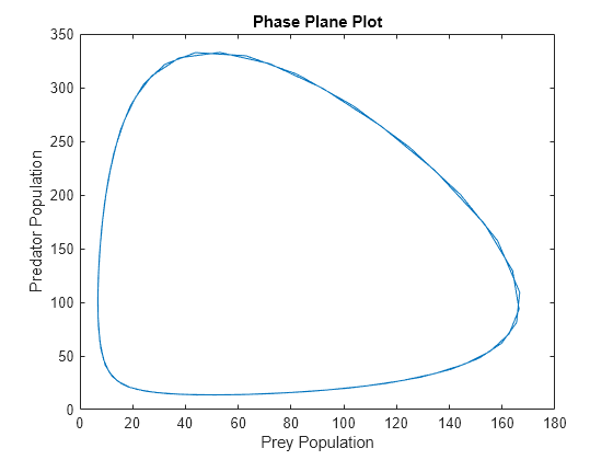
现在绘制两个种群数量的相对关系图。生成的相平面图非常清晰地表明了二者数量之间的循环关系。
plot(y(1,:),y(2,:))
title("Phase Plane Plot")
xlabel("Prey Population")
ylabel("Predator Population")
比较不同求解器的结果
使用 ode45 求解器而不是 ode23 求解器再次求解方程组。ode45 求解器的每一步都需要更长的时间,但它的步长也更大。然而,ode45 的输出是平滑的,因为默认情况下,此求解器使用连续展开公式在每个步长范围内的四个等间距时间点生成输出。(您可以使用 solve 方法的 Refine 名称-值参量来调整时间点数。)绘制两个解进行比较。
F.Solver = "ode45";
S2 = solve(F,t0,tfinal);
t2 = S2.Time;
y2 = S2.Solution;

plot(y(1,:),y(2,:),"o",y2(1,:),y2(2,:),".");
title("Phase Plane Plot")
legend("ode23","ode45")
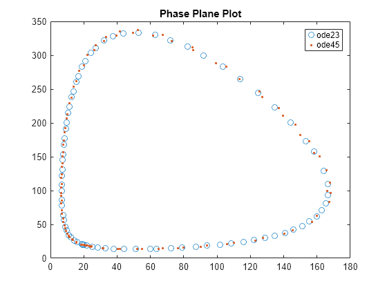
结果表明,使用不同的数值方法求解微分方程会产生略微不同的答案。