求解具有强状态相关质量矩阵的 ODE

此示例说明如何使用移动网格方法求解伯格斯方程 [1]。该问题包括质量矩阵，并指定了选项来描述质量矩阵的强状态依赖性和稀疏性，使求解过程更加高效。

问题设置

伯格斯方程是一种对流扩散方程，由以下 PDE 给出

$\frac{\partial u}{\partial t} = ϵ \frac{\partial^{2} u}{{\partial x}^{2}} - \frac{\partial}{\partial x} (\frac{u^{2}}{2}), 0 < x < 1, t > 0, ϵ = 1 {\times 10}^{- 4} .$

应用坐标变换（[1] 中的方程 18）会使左侧出现额外的项：

$\frac{\partial u}{\partial t} - \frac{\partial u}{\partial x} \frac{\partial x}{\partial t} = ϵ \frac{\partial^{2} u}{{\partial x}^{2}} - \frac{\partial}{\partial x} (\frac{u^{2}}{2}) .$

通过使用有限差分逼近关于 $x$ 的偏导数可将 PDE 转换为仅有一个变量的 ODE。如果有限差分写为 $Δ$ ，则 PDE 可以重写为只包含关于 $t$ 的导数的 ODE：

$\frac{du}{dt} - Δ u \frac{dx}{dt} = ϵ Δ^{2} u - Δ (\frac{u^{2}}{2}) .$

在此形式中，您可以使用 ODE 求解器（如 ode15s）来求解 $u$ 和 $x$ 随时间的变化。

对于此示例，问题由包含 $N$ 个点的移动网格表示，[1] 中所述的移动网格方法在每个时间步定位网格点，使它们始终集中在变化区域。边界和初始条件是

$\begin{array}{l} u (0, t) = u (1, t) = 0, \\ u (x, 0) = \sin (2 π x) + \frac{1}{2} \sin (π x) . \end{array}$

对于由 $N$ 个点组成的给定初始网格，有 $2 N$ 个方程需要求解： $N$ 个方程对应于伯格斯方程，另外 $N$ 个方程确定每个网格点的运动。因此，最终的方程组是：

$\begin{array}{l} \frac{d u_{1}}{dt} - Δ u_{1} \frac{d x_{1}}{dt} = ϵ Δ^{2} u_{1} - Δ (\frac{{u_{1}}^{2}}{2}), \\ ⋮ \\ \frac{d u_{N}}{dt} - Δ u_{N} \frac{d x_{N}}{dt} = ϵ Δ^{2} u_{N} - Δ (\frac{{u_{N}}^{2}}{2}), \\ \frac{d^{2} {x_{1}}_{}^{˙}}{d t^{2}} = \frac{1}{τ} \frac{d}{dt} (B (x_{1}, t) \frac{d x_{1}}{dt}), \\ ⋮ \\ \frac{d^{2} {x_{N}}_{}^{˙}}{d t^{2}} = \frac{1}{τ} \frac{d}{dt} (B (x_{N}, t) \frac{d x_{N}}{dt}) . \end{array}$

移动网格的项对应于 [1] 中的 MMPDE6。参数 $τ$ 表示强制网格趋向均匀分布的时间刻度。项 $B (x, t)$ 是由[1] 中的方程 21 给出的监控函数：

$B (x, t) = \sqrt{1 + {(\frac{d u_{i}}{d x_{i}})}^{2}} .$

此示例中使用的通过移动网格点求解伯格斯方程方程的方式展示了几种方法：

方程组用质量矩阵公式表示， $M y^{'} = f (t, y)$ 。质量矩阵作为函数提供给 ode15s 求解器。
导函数不仅包括表示伯格斯方程的方程，还包括一组控制移动网格选择的方程。
雅可比 $dF / dy$ 的稀疏模式和质量矩阵的导数乘以向量 $d (Mv) / dy$ 作为函数提供给求解器。提供这些稀疏模式有助于求解器更高效地运行。
有限差分用于逼近几个偏导数。

要在 MATLAB® 中求解此方程，请编写导函数、质量矩阵函数、雅可比 $dF / dy$ 的稀疏模式的函数以及 $d (Mv) / dy$ 的稀疏模式的函数。您可以将所需的函数作为局部函数包含在文件末尾（如本处所示），或者将它们作为单独的命名文件保存在 MATLAB 路径上的目录中。

编写质量矩阵代码

方程组的左侧涉及一阶导数的线性组合，因此需要质量矩阵来表示所有项。将方程组的左侧设置为等于 $M y^{'}$ 以提取质量矩阵的形式。质量矩阵由四个分块组成，每个分块均为 $N$ 阶方阵：

$[\begin{array}{c} \frac{\partial u_{1}}{\partial t} - \frac{\partial u_{1}}{\partial x_{1}} \frac{\partial x_{1}}{\partial t} \\ ⋮ \\ \frac{\partial u_{N}}{\partial t} - \frac{\partial u_{N}}{\partial x_{N}} \frac{\partial x_{N}}{\partial t} \\ \frac{\partial^{2} {x_{1}}_{}^{˙}}{\partial t^{2}} \\ ⋮ \\ \frac{\partial^{2} {x_{N}}_{}^{˙}}{\partial t^{2}} \end{array}] = M y^{'} = [\begin{array}{cc} M_{1} & M_{2} \\ M_{3} & M_{4} \end{array}] [\begin{array}{c} {u_{1}}_{}^{˙} \\ ⋮ \\ {u_{N}}_{}^{˙} \\ {x_{1}}_{}^{˙} \\ ⋮ \\ {x_{N}}_{}^{˙} \end{array}]$ .

此公式表明， $M_{1}$ 和 $M_{2}$ 构成伯格斯方程的左侧（方程组中的前 $N$ 个方程），而 $M_{3}$ 和 $M_{4}$ 构成网格方程的左侧（方程组中的最后 $N$ 个方程）。分块矩阵是：

$\begin{array}{l} M_{1} = I_{N}, \\ M_{2} = - \frac{\partial u_{i}}{\partial x_{i}} I_{N}, \\ M_{3} = 0_{N}, \\ M_{4} = \frac{\partial^{2}}{\partial t^{2}} I_{N} . \end{array}$

$I_{N}$ 是 $N \times N$ 单位矩阵。 $M_{2}$ 中的偏导数是使用有限差分估计的，而 $M_{4}$ 中的偏导数使用拉普拉斯矩阵。请注意， $M_{3}$ 只包含零，因为网格移动的所有方程都不依赖于 $u_{}^{˙}$ 。

现在您可以编写一个用于计算质量矩阵的函数。该函数必须接受时间 $t$ 和解向量 $y$ 两个输入。由于解向量 $y$ 包含一半 $u_{}^{˙}$ 分量和一半 $x_{}^{˙}$ 分量，该函数首先提取这些分量。然后，该函数构建所有分块矩阵（考虑问题的边界值），并使用四个分块组合成质量矩阵。

function M = mass(t,y)
% Extract the components of y for the solution u and mesh x
N = length(y)/2; 
u = y(1:N);
x = y(N+1:end);

% Boundary values of solution u and mesh x
u0 = 0;
uNP1 = 0;
x0 = 0;
xNP1 = 1;

% M1 and M2 are the portions of the mass matrix for Burgers' equation. 
% The derivative du/dx is approximated with finite differences, using 
% single-sided differences on the edges and centered differences in between.
M1 = speye(N);
i = 2:N-1;
v = [0; -(u(i+1) - u(i-1))./(x(i+1) - x(i-1)) ; 0];
M2 = spdiags(v,0,N,N);

M2(1,1) = - (u(2) - u0)/(x(2) - x0);
M2(N,N) = - (uNP1 - u(N-1))/(xNP1 - x(N-1));

% M3 and M4 define the equations for mesh point evolution, corresponding to 
% MMPDE6 in the reference paper. Since the mesh functions only involve d/dt(dx/dt), 
% the M3 portion of the mass matrix is all zeros. The second derivative in M4 is 
% approximated using a finite difference Laplacian matrix. 
M3 = sparse(N,N);
M4 = spdiags([1 -2 1],-1:1,N,N);

% Assemble mass matrix
M = [M1 M2; M3 M4];
end

注意：所有函数都作为局部函数包含在示例的末尾。

编写导函数代码

此问题的导函数返回一个包含 $2 N$ 个元素的向量。前 $N$ 个元素对应于伯格斯方程，而后 $N$ 个元素对应于移动网格方程。函数 movingMeshODE 通过这些步骤来计算方程组中所有方程的右侧：

使用有限差分（前 $N$ 个元素）计算伯格斯方程。
计算监控函数（最后 $N$ 个元素）。
应用空间平滑处理来监控函数和计算移动网格方程。

导函数中的前 $N$ 个方程对伯格斯方程的右侧进行编码。伯格斯方程可视为微分运算子，涉及以下形式的空间导数：

$f (u) = ϵ \frac{\partial^{2} u}{{\partial x}^{2}} - \frac{\partial}{\partial x} (\frac{u^{2}}{2})$ .

参考文献 [1] 通过以下公式说明使用中心有限差分逼近微分运算子 $f$ 的过程

$f_{i} = ϵ [\frac{(\frac{u_{i + 1} - u_{i}}{x_{i + 1} - x_{i}}) - (\frac{u_{i} - u_{i - 1}}{x_{i} - x_{i - 1}})}{\frac{1}{2} (x_{i + 1} - x_{i - 1})}] - \frac{1}{2} (\frac{u_{i + 1}^{2} - u_{i - 1}^{2}}{x_{i + 1} - x_{i - 1}}) .$

在网格的边缘（此时 $i = 1$ 和 $i = N$ ），仅使用单侧差分。此示例使用 $ϵ = 1 \times 10^{- 4}$ 。

控制网格的方程（包括导函数中的最后 $N$ 个方程）是

$\frac{\partial^{2} x_{}^{˙}}{\partial t^{2}} = \frac{1}{τ} \frac{\partial}{\partial t} (B (x, t) \frac{\partial x}{\partial t}) .$

就像对伯格斯方程一样，您可以使用有限差分来逼近监控函数 $B (x, t)$ ：

$B (x, t) = \sqrt{1 + {(\frac{\partial u_{i}}{\partial x_{i}})}^{2}} = \sqrt{1 + {(\frac{u_{i + 1} - u_{i - 1}}{x_{i + 1} - x_{i - 1}})}^{2}} .$

计算监控函数后，应用空间平滑处理（[1] 中的方程 14 和 15）。此示例使用 $γ = 2$ 和 $p = 2$ 作为空间平滑处理参数。

对方程组进行编码的函数是

function g = movingMeshODE(t,y)
% Extract the components of y for the solution u and mesh x
N = length(y)/2;
u = y(1:N);
x = y(N+1:end);

% Boundary values of solution u and mesh x
u0 = 0;
uNP1 = 0;
x0 = 0;
xNP1 = 1;

% Preallocate g vector of derivative values.
g = zeros(2*N,1);

% Use centered finite differences to approximate the RHS of Burgers'
% equations (with single-sided differences on the edges). The first N
% elements in g correspond to Burgers' equations.
ind = 1:N;
x = [x0; x; xNP1];
u = [u0; u; uNP1];
i = 2:N+1;
delx = x(i+1) - x(i-1);
g(ind) = 1e-4*((u(i+1) - u(i))./(x(i+1) - x(i)) - ...
          (u(i) - u(i-1))./(x(i) - x(i-1)))./(0.5*delx) - ...
          0.5*(u(i+1).^2 - u(i-1).^2)./delx;

% Evaluate the monitor function values (Eq. 21 in reference paper), used in
% RHS of mesh equations. Centered finite differences are used for interior
% points, and single-sided differences are used on the edges.
M = zeros(N,1);
M(ind) = sqrt(1 + ((u(i+1) - u(i-1))./(x(i+1) - x(i-1))).^2);
M0 = sqrt(1 + ((u(2) - u0)/(x(2) - x0))^2);
MNP1 = sqrt(1 + ((uNP1 - u(N+1))/(xNP1 - x(N+1)))^2);

% Apply spatial smoothing (Eqns. 14 and 15) with gamma = 2, p = 2.
x = y(N+1:end);
ind = 2:N-1;
SM = zeros(N,1);
i = 3:N-2;
SM(i) = sqrt((4*M(i-2).^2 + 6*M(i-1).^2 + 9*M(i).^2 + ...
    6*M(i+1).^2 + 4*M(i+2).^2)/29);

SM0 = sqrt((9*M0^2 + 6*M(1)^2 + 4*M(2)^2)/19);
SM(1) = sqrt((6*M0^2 + 9*M(1)^2 + 6*M(2)^2 + 4*M(3)^2)/25);
SM(2) = sqrt((4*M0^2 + 6*M(1)^2 + 9*M(2)^2 + 6*M(3)^2 + 4*M(4)^2)/29);
SM(N-1) = sqrt((4*M(N-3)^2 + 6*M(N-2)^2 + 9*M(N-1)^2 + 6*M(N)^2 + 4*MNP1^2)/29);
SM(N) = sqrt((4*M(N-2)^2 + 6*M(N-1)^2 + 9*M(N)^2 + 6*MNP1^2)/25);
SMNP1 = sqrt((4*M(N-1)^2 + 6*M(N)^2 + 9*MNP1^2)/19);

g(ind+N) = (SM(ind+1) + SM(ind)).*(x(ind+1) - x(ind)) - ...
    (SM(ind) + SM(ind-1)).*(x(ind) - x(ind-1));
g(1+N) = (SM(2) + SM(1))*(x(2) - x(1)) - (SM(1) + SM0)*(x(1) - x0);
g(N+N) = (SMNP1 + SM(N))*(xNP1 - x(N)) - (SM(N) + SM(N-1))*(x(N) - x(N-1));

% Form final discrete approximation for Eq. 12 in reference paper, the equation governing
% the mesh points.
tau = 1e-3;
g(1+N:end) = - g(1+N:end)/(2*tau);
end

编写稀疏模式函数的代码

导函数的雅可比 $dF / dy$ 是 $2 N \times 2 N$ 矩阵，其中包含导函数 movingMeshODE 的所有偏导数。当 options 结构体中没有提供矩阵时，ode15s 使用有限差分估计雅可比矩阵。您可以提供雅可比矩阵的稀疏模式来帮助 ode15s 更快地计算它。

雅可比矩阵稀疏模式的函数是

function out = JPat(N)
S1 = spdiags(1,-1:1,N,N);
S2 = spdiags(1,-4:4,N,N);
out = [S1 S1; S2 S2];
end

使用 spy 绘制 $N = 80$ 的 $dF / dy$ 稀疏模式。

spy(JPat(80))

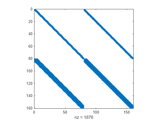
Figure contains an axes object. The axes object with xlabel nz = 1876 contains a line object which displays its values using only markers.

另一种提高计算效率的方法是提供 $d (Mv) / dy$ 的稀疏模式。通过检查在质量矩阵函数中计算的有限差分中存在 $u_{i}$ 和 $x_{i}$ 的哪些项，可以找到这种稀疏模式。

用于计算 $d (Mv) / dy$ 的稀疏模式的函数是

function S = MvPat(N)
SZ = sparse(N,N);
S1 = spdiags(1,[-1 1],N,N);
S = [S1 S1; SZ SZ];
end

使用 spy 绘制 $N = 80$ 的 $d (Mv) / dy$ 稀疏模式。

spy(MvPat(80))

Figure contains an axes object. The axes object with xlabel nz = 316 contains a line object which displays its values using only markers.

求解方程组

用值 $N = 80$ 求解方程组。对于初始条件，用均匀网格初始化 $x$ ，并在网格上计算 $u (x, 0)$ 。

N = 80;
h = 1/(N+1);
xinit = h*(1:N);
uinit = sin(2*pi*xinit) + 0.5*sin(pi*xinit);
y0 = [uinit xinit];

使用 odeset 创建一个 options 结构体，该结构体设置多个值：

质量矩阵的函数句柄
质量矩阵的状态依赖性，对于此问题是 'strong'，因为质量矩阵是 $t$ 和 $y$ 两者的函数
用于计算雅可比稀疏模式的函数句柄
用于计算质量矩阵的导数并乘以向量的稀疏模式的函数句柄
绝对和相对误差容限

opts = odeset(Mass=@mass,MStateDependence="strong",JPattern=JPat(N),...
       MvPattern=MvPat(N),RelTol=1e-5,AbsTol=1e-4);

最后，调用 ode15s 以使用 movingMeshODE 导函数、时间跨度、初始条件和 options 结构体在区间 $[0, 1]$ 上求解方程组。

tspan = [0 1];
sol = ode15s(@movingMeshODE,tspan,y0,opts);

绘制结果

积分的结果是结构体 sol，其中包含时间步 $t$ 、网格点 $x (t)$ 和解 $u (x, t)$ 。从结构体中提取这些值。

t = sol.x;
x = sol.y(N+1:end,:);
u = sol.y(1:N,:);

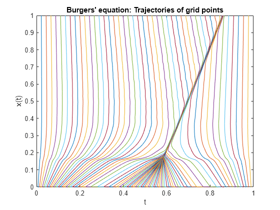
绘制网格点随时间的移动。该图显示，随着时间的推移，网格点保持合理的均匀间距（由于监控函数的作用），但这些网格点能够移向并聚集在解的不连续点附近。

plot(x,t)
xlabel("t")
ylabel("x(t)")
title("Burgers' equation: Trajectories of grid points")

Figure contains an axes object. The axes object with title Burgers' equation: Trajectories of grid points, xlabel t, ylabel x(t) contains 80 objects of type line.

现在，在 $t$ 的几个值上对 $u (x, t)$ 进行采样，并绘制解随时间的演变图。区间末端的网格点是固定的，即 x(0) = 0 和 x(N+1) = 1。边界值为 u(t,0) = 0 和 u(t,1) = 0，您必须将其添加到为该图计算的已知值中。

tint = 0:0.2:1;
yint = deval(sol,tint);
figure
labels = {};
for j = 1:length(tint)
   solution = [0; yint(1:N,j); 0];
   location = [0; yint(N+1:end,j); 1];
   labels{j} = ['t = ' num2str(tint(j))];
   plot(location,solution,"-o")
   hold on
end
xlabel("x")
ylabel("solution u(x,t)")
legend(labels{:},"Location","SouthWest")
title("Burgers equation on moving mesh")
hold off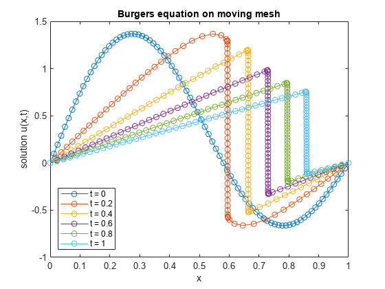

Figure contains an axes object. The axes object with title Burgers equation on moving mesh, xlabel x, ylabel solution u(x,t) contains 6 objects of type line. These objects represent t = 0, t = 0.2, t = 0.4, t = 0.6, t = 0.8, t = 1.

该图显示 $u (x, 0)$ 是平滑的波形，随着时间的推移，它会向 $x = 1$ 移动，形成陡峭的梯度。网格点跟踪不连续点的移动，以便在每个时间步中额外的计算点位于适当的位置。

参考

[1] Huang, Weizhang, et al.“Moving Mesh Methods Based on Moving Mesh Partial Differential Equations.”Journal of Computational Physics, vol. 113, no. 2, Aug. 1994, pp. 279–90. https://doi.org/10.1006/jcph.1994.1135.

局部函数

此处列出了求解器 ode15s 为计算解而调用的局部辅助函数。您也可以将这些函数作为它们自己的文件保存在 MATLAB 路径上的目录中。

function g = movingMeshODE(t,y)
% Extract the components of y for the solution u and mesh x
N = length(y)/2;
u = y(1:N);
x = y(N+1:end);

% Boundary values of solution u and mesh x
u0 = 0;
uNP1 = 0;
x0 = 0;
xNP1 = 1;

% Preallocate g vector of derivative values.
g = zeros(2*N,1);

% Use centered finite differences to approximate the RHS of Burgers'
% equations (with single-sided differences on the edges). The first N
% elements in g correspond to Burgers' equations.
ind = 1:N;
x = [x0; x; xNP1];
u = [u0; u; uNP1];
i = 2:N+1;
delx = x(i+1) - x(i-1);
g(ind) = 1e-4*((u(i+1) - u(i))./(x(i+1) - x(i)) - ...
          (u(i) - u(i-1))./(x(i) - x(i-1)))./(0.5*delx) - ...
          0.5*(u(i+1).^2 - u(i-1).^2)./delx;

% Evaluate the monitor function values (Eq. 21 in reference paper), used in
% RHS of mesh equations. Centered finite differences are used for interior
% points, and single-sided differences are used on the edges.
M = zeros(N,1);
M(ind) = sqrt(1 + ((u(i+1) - u(i-1))./(x(i+1) - x(i-1))).^2);
M0 = sqrt(1 + ((u(2) - u0)/(x(2) - x0))^2);
MNP1 = sqrt(1 + ((uNP1 - u(N+1))/(xNP1 - x(N+1)))^2);

% Apply spatial smoothing (Eqns. 14 and 15) with gamma = 2, p = 2.
x = y(N+1:end);
ind = 2:N-1;
SM = zeros(N,1);
i = 3:N-2;
SM(i) = sqrt((4*M(i-2).^2 + 6*M(i-1).^2 + 9*M(i).^2 + ...
    6*M(i+1).^2 + 4*M(i+2).^2)/29);

SM0 = sqrt((9*M0^2 + 6*M(1)^2 + 4*M(2)^2)/19);
SM(1) = sqrt((6*M0^2 + 9*M(1)^2 + 6*M(2)^2 + 4*M(3)^2)/25);
SM(2) = sqrt((4*M0^2 + 6*M(1)^2 + 9*M(2)^2 + 6*M(3)^2 + 4*M(4)^2)/29);
SM(N-1) = sqrt((4*M(N-3)^2 + 6*M(N-2)^2 + 9*M(N-1)^2 + 6*M(N)^2 + 4*MNP1^2)/29);
SM(N) = sqrt((4*M(N-2)^2 + 6*M(N-1)^2 + 9*M(N)^2 + 6*MNP1^2)/25);
SMNP1 = sqrt((4*M(N-1)^2 + 6*M(N)^2 + 9*MNP1^2)/19);

g(ind+N) = (SM(ind+1) + SM(ind)).*(x(ind+1) - x(ind)) - ...
    (SM(ind) + SM(ind-1)).*(x(ind) - x(ind-1));
g(1+N) = (SM(2) + SM(1))*(x(2) - x(1)) - (SM(1) + SM0)*(x(1) - x0);
g(N+N) = (SMNP1 + SM(N))*(xNP1 - x(N)) - (SM(N) + SM(N-1))*(x(N) - x(N-1));

% Form final discrete approximation for Eq. 12 in reference paper, the equation governing
% the mesh points.
tau = 1e-3;
g(1+N:end) = - g(1+N:end)/(2*tau);
end

% -----------------------------------------------------------------------
function M = mass(t,y)
% Extract the components of y for the solution u and mesh x
N = length(y)/2; 
u = y(1:N);
x = y(N+1:end);

% Boundary values of solution u and mesh x
u0 = 0;
uNP1 = 0;
x0 = 0;
xNP1 = 1;

% M1 and M2 are the portions of the mass matrix for Burgers' equation. 
% The derivative du/dx is approximated with finite differences, using 
% single-sided differences on the edges and centered differences in between.
M1 = speye(N);
i = 2:N-1;
v = [0; -(u(i+1) - u(i-1))./(x(i+1) - x(i-1)) ; 0];
M2 = spdiags(v,0,N,N);

M2(1,1) = - (u(2) - u0)/(x(2) - x0);
M2(N,N) = - (uNP1 - u(N-1))/(xNP1 - x(N-1));

% M3 and M4 define the equations for mesh point evolution, corresponding to 
% MMPDE6 in the reference paper. Since the mesh functions only involve d/dt(dx/dt), 
% the M3 portion of the mass matrix is all zeros. The second derivative in M4 is 
% approximated using a finite difference Laplacian matrix. 
M3 = sparse(N,N);
M4 = spdiags([1 -2 1],-1:1,N,N);

% Assemble mass matrix
M = [M1 M2; M3 M4];
end

% -------------------------------------------------------------------------
function out = JPat(N)  % Jacobian sparsity pattern
S1 = spdiags(1,-1:1,N,N);
S2 = spdiags(1,-4:4,N,N);
out = [S1 S1; S2 S2];
end

% -------------------------------------------------------------------------
function S = MvPat(N)  % Sparsity pattern for the derivative of the Mass matrix times a vector
SZ = sparse(N,N);
S1 = spdiags(1,[-1 1],N,N);
S = [S1 S1; SZ SZ];
end
% -------------------------------------------------------------------------

另请参阅

ode15s | odeset