沃罗诺伊图
离散点集 X 的沃罗诺伊图将每个点 X(i) 周围的空间分解成影响区域 R{i}。这种分解具有的属性是区域 R{i} 中的任意点 P 比任何其他点更靠近点 i。这种影响区域称为沃罗诺伊区域,所有沃罗诺伊区域的集合构成沃罗诺伊图。
沃罗诺伊图是一个 N 维几何结构,但是大多数实际应用程序是位于二维和三维空间中的。使用一个示例最好理解沃罗诺伊图的属性。
绘图二维沃罗诺伊图和德劳内三角剖分
本示例在同一个二维图上显示沃罗诺伊图和德劳内三角剖分。
使用二维 voronoi 函数绘制某一点集的沃罗诺伊图。
figure()
X = [-1.5 3.2; 1.8 3.3; -3.7 1.5; -1.5 1.3; ...
      0.8 1.2; 3.3 1.5; -4.0 -1.0;-2.3 -0.7; ...
      0 -0.5; 2.0 -1.5; 3.7 -0.8; -3.5 -2.9; ...
     -0.9 -3.9; 2.0 -3.5; 3.5 -2.25];

voronoi(X(:,1),X(:,2))

% Assign labels to the points.
nump = size(X,1);
plabels = arrayfun(@(n) {sprintf('X%d', n)}, (1:nump)');
hold on
Hpl = text(X(:,1), X(:,2), plabels, 'FontWeight', ...
      'bold', 'HorizontalAlignment','center', ...
      'BackgroundColor', 'none');

% Add a query point, P, at (0, -1.5).
P = [0 -1];
plot(P(1),P(2), '*r');
text(P(1), P(2), 'P', 'FontWeight', 'bold', ...
     'HorizontalAlignment','center', ...
     'BackgroundColor', 'none');
hold off
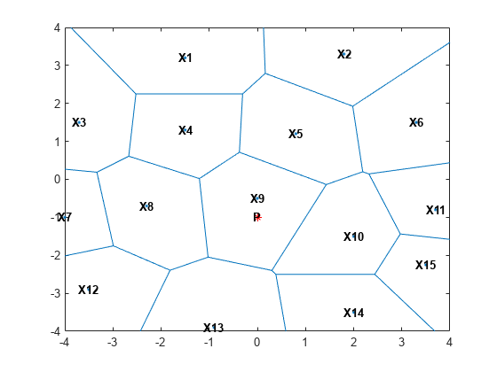
观察发现 P 比 X 中的任何其他点更靠近 X9,对于约束 X9 的区域中的任何点 P 都是如此。
点集 X 的沃罗诺伊图与 X 的德劳内三角剖分密切相关。要了解这种关系,请构建点集 X 的一个德劳内三角剖分,然后在沃罗诺伊图上叠加该三角剖分图。
dt = delaunayTriangulation(X);
hold on
triplot(dt,'-r');
hold off
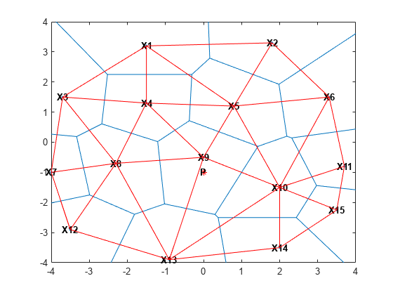
从图上可以看出,与点 X9 相关联的沃罗诺伊区域由连接到 X9 的德劳内边的垂直平分线确定。此外,沃罗诺伊边的顶点位于德劳内三角形的外接圆心处。通过绘出三角形 {|X9|,|X4|,|X8|} 的外接圆心,可以说明这些联系。
为求出此三角形的索引,请查询三角剖分。此三角形包含位置 (-1, 0)。
tidx = pointLocation(dt,-1,0);
现在,求出此三角形的外接圆心,并用绿色绘图。
cc = circumcenter(dt,tidx);
hold on
plot(cc(1),cc(2),'*g');
hold off
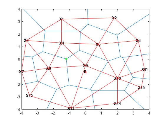
德劳内三角剖分和沃罗诺伊图互为几何对偶。从德劳内三角剖分可以计算沃罗诺伊图,反之亦然。
观察与凸包上的点相关联的沃罗诺伊区域是否是无界的(例如与 X13 相关联的沃罗诺伊区域)。此区域中的边“终止”于无穷远处。平分德劳内边 (X13, X12) 和 (X13, X14) 的沃罗诺伊边延伸至无穷远处。虽然沃罗诺伊图提供了点集中每个点附近空间的最近邻点分解,但是不直接支持最近邻点查询。然而,用于计算沃罗诺伊图的几何结构也用于执行最近邻点搜索。
计算沃罗诺伊图
本示例显示如何计算二维和三维沃罗诺伊图。
MATLAB® 提供用于绘制二维沃罗诺伊图以及计算 N 维沃罗诺伊图的拓扑的函数。事实上,由于所需内存的指数级增长,对高于六维的大中型数据集,沃罗诺伊计算是不实际的。
voronoi 绘图函数为二维空间的点集绘制沃罗诺伊图。在 MATLAB 中,有两种方式计算点集的沃罗诺伊图:
使用函数
voronoin
voronoin 函数支持为 N 维空间 (N ≥ 2) 中的离散点计算沃罗诺伊拓扑。voronoiDiagram 方法支持为二维或三维离散点计算沃罗诺伊拓扑。
建议用 voronoiDiagram 方法计算二维或三维拓扑,因为此方法更稳定,对大型数据集表现更佳。此方法支持递增插值、移除点和补充查询,例如最近邻点搜索。
voronoin 函数和 voronoiDiagram 方法使用矩阵格式表示沃罗诺伊图的拓扑。有关此数据结构的详细信息,请参阅 三角剖分矩阵格式。
计算沃罗诺伊图
此示例说明如何计算二维和三维沃罗诺伊图。
给定点集 X,按如下方式获取沃罗诺伊图的拓扑:
使用
voronoin函数
[V,R] = voronoin(X)
使用
voronoiDiagram方法
dt = delaunayTriangulation(X);
[V,R] = voronoiDiagram(dt)
V 是表示沃罗诺伊顶点(这些顶点是沃罗诺伊边的端点)坐标的矩阵。按照惯例,V 中的第一个顶点是无限顶点。R 是向量元胞数组长度 size(X,1),表示与每个点相关联的沃罗诺伊区域。因此,与点 X(i) 相关联的沃罗诺伊区域是 R{i}。
定义点集并绘制其沃罗诺伊图
X = [-1.5 3.2; 1.8 3.3; -3.7 1.5; -1.5 1.3; 0.8 1.2; ...
      3.3 1.5; -4.0 -1.0; -2.3 -0.7; 0 -0.5; 2.0 -1.5; ...
      3.7 -0.8; -3.5 -2.9; -0.9 -3.9; 2.0 -3.5; 3.5 -2.25];
[VX,VY] = voronoi(X(:,1),X(:,2));
h = plot(VX,VY,"-b",X(:,1),X(:,2),".r");
xlim([-4 4])
ylim([-4 4])

% Assign labels to the points X.
nump = size(X,1);
plabels = arrayfun(@(n) {sprintf('X%d', n)},(1:nump)');
hold on
Hpl = text(X(:,1),X(:,2)+0.2,plabels,color="r",FontWeight="bold", ...
    HorizontalAlignment="center",BackgroundColor="none");

% Compute the Voronoi diagram.
dt = delaunayTriangulation(X);
[V,R] = voronoiDiagram(dt);


% Assign labels to the Voronoi vertices V.
% By convention the first vertex is at infinity.
numv = size(V,1);
vlabels = arrayfun(@(n) {sprintf("V%d", n)},(2:numv)');
hold on
Hpl = text(V(2:end,1),V(2:end,2)+.2,vlabels,FontWeight="bold", ...
    HorizontalAlignment="center",BackgroundColor="none");
hold off
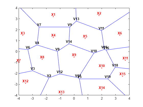
R{9} 给出了与点位 X9 相关联的沃罗诺伊顶点的索引。
R{9}ans = 1×5
8 12 17 10 14
沃罗诺伊顶点的索引是基于 V 数组的索引。
类似地,R{4} 给出了与点位 X4 相关联的沃罗诺伊顶点的索引。
R{4}ans = 1×5
4 8 14 9 7
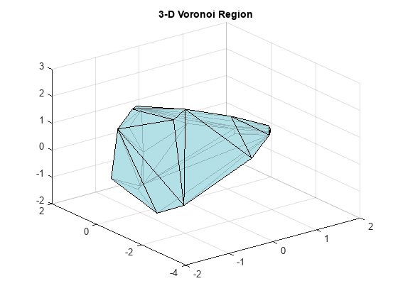
在三维空间中,沃罗诺伊区域为凸多面体,创建沃罗诺伊图的语法是相似的。但沃罗诺伊图的几何形状更加复杂。以下示例描述了三维沃罗诺伊图的创建过程和单个区域的绘制过程。
在三维空间创建一个包含 25 个点的样本,并计算此点集的沃罗诺伊图的拓扑。
rng("default")
X = -3 + 6.*rand([25 3]);
dt = delaunayTriangulation(X);
计算沃罗诺伊图的拓扑。
[V,R] = voronoiDiagram(dt);
求距离原点最近的点,并绘制与此点相关联的沃罗诺伊区域。
tid = nearestNeighbor(dt,0,0,0);
XR10 = V(R{tid},:);
K = convhull(XR10);
defaultFaceColor = [0.6875 0.8750 0.8984];
trisurf(K,XR10(:,1),XR10(:,2),XR10(:,3) , ...
        FaceColor=defaultFaceColor,FaceAlpha=0.8)
title("3-D Voronoi Region")