Main Content

islocalmin2

Find local minima in 2-D data

Since R2024a

Description

TF = islocalmin2(A) returns a logical array whose elements are 1 (true) when a local minimum is detected in the corresponding element of A.

example

[TF,P] = islocalmin2(A) also returns the prominence corresponding to each element of A. For more information about the prominence calculation, see Algorithms.

example

___ = islocalmin2(A,Name=Value) specifies options for finding local minima using one or more name-value arguments with either of the output argument combinations in the previous syntaxes. For example, TF = islocalmin2(A,MaxNumExtrema=4) finds no more than four of the most prominent local minima.

example

Examples

collapse all

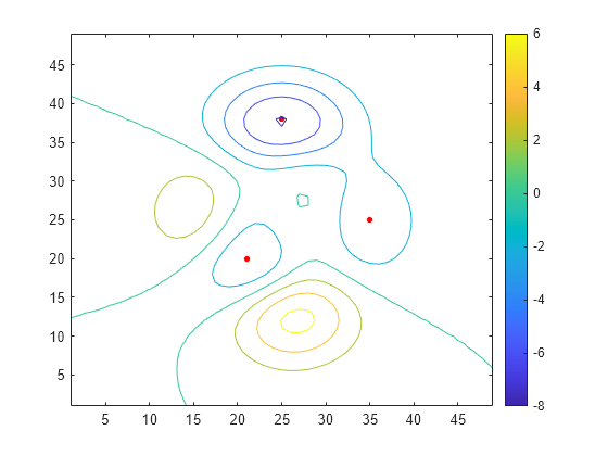
Create a matrix, and visualize the matrix using a contour plot.

A = -peaks;
contour(A)
colorbar

Figure contains an axes object. The axes object contains an object of type contour.

Determine the locations of the local minima.

TF = islocalmin2(A);

Use the local minima indicator to determine the value of each minimum.

minval = A(TF)
minval = 3×1

   -3.7573
   -8.0752
   -3.5823

Plot the local minima on the contour plot.

[X,Y] = meshgrid(1:49,1:49);
hold on
plot3(X(TF),Y(TF),minval,"red.",MarkerSize=12)

Figure contains an axes object. The axes object contains 2 objects of type contour, line. One or more of the lines displays its values using only markers

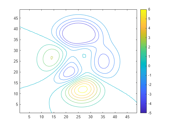
Create and visualize a matrix with a flat region.

data = -peaks;
A = clip(data,-5,Inf);
contour(A)
colorbar

Figure contains an axes object. The axes object contains an object of type contour.

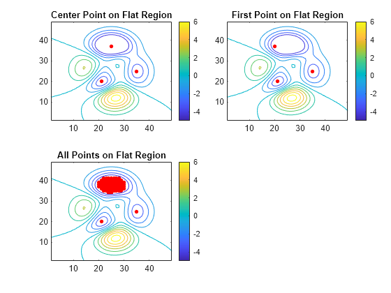
Find the local minima. By default, TF is 1 (true) for only the center point of the flat region and TF is 0 (false) for all other points on the flat region.

[TF,P] = islocalmin2(A);

To select only the point on the flat region with the smallest linear index as the local minimum, specify the FlatSelection name-value argument as "first".

[TF2,P2] = islocalmin2(A,FlatSelection="first");

To select all points on the flat region as local minima, specify FlatSelection as "all".

[TF3,P3] = islocalmin2(A,FlatSelection="all");

Compare the results of the flat region selections by visualizing the extrema.

[X,Y] = meshgrid(1:49,1:49);
tiledlayout(2,2)

nexttile
contour(A)
colorbar
hold on
plot3(X(TF),Y(TF),A(TF),"red.",MarkerSize=12)
title("Center Point on Flat Region")

nexttile
contour(A)
colorbar
hold on
plot3(X(TF2),Y(TF2),A(TF2),"red.",MarkerSize=12)
title("First Point on Flat Region")

nexttile
contour(A)
colorbar
hold on
plot3(X(TF3),Y(TF3),A(TF3),"red.",MarkerSize=12)
title("All Points on Flat Region")

Figure contains 3 axes objects. Axes object 1 with title Center Point on Flat Region contains 2 objects of type contour, line. One or more of the lines displays its values using only markers Axes object 2 with title First Point on Flat Region contains 2 objects of type contour, line. One or more of the lines displays its values using only markers Axes object 3 with title All Points on Flat Region contains 2 objects of type contour, line. One or more of the lines displays its values using only markers

Only the local minima indicator changes when you specify FlatSelection. The prominence of all data points is the same for all values of FlatSelection.

isequal(P,P2,P3)
ans = logical
   1

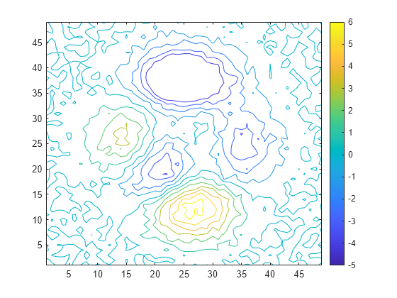
Create a matrix with some noise, and visualize the matrix using a contour plot.

data = peaks;
data = -data - randn(49)*0.3;
A = clip(data,-5,Inf);

contour(A)
colorbar

Figure contains an axes object. The axes object contains an object of type contour.

Find the local minima and plot them on the contour plot. By default, islocalmin2 finds all local minima whose prominence is greater than 0.

[TF P] = islocalmin2(A);

To understand the prominence of the local minima, sort the unique prominence values.

maxP = sort(unique(P(:)),"descend")
maxP = 143×1

    5.7516
    3.9830
    3.3811
    2.6829
    1.7200
    1.2871
    1.2853
    1.1382
    1.1128
    1.0921
      ⋮

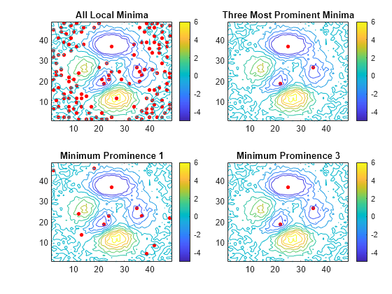
Ignore the local minima that are a result of noise by finding only the three most prominent local minima. When you specify the MaxNumExtrema name-value argument, the points in a flat region are jointly considered a single minimum point.

TF2 = islocalmin2(A,MaxNumExtrema=3);

Find local minima whose prominence is greater than 1.

TF3 = islocalmin2(A,MinProminence=1);

Find local minima whose prominence is greater than 3.

TF4 = islocalmin2(A,MinProminence=3);

Compare the results of the prominence filters by visualizing the extrema.

[X,Y] = meshgrid(1:49,1:49);
figure
tiledlayout(2,2)

nexttile
contour(A)
colorbar
hold on
plot3(X(TF),Y(TF),A(TF),"r.",MarkerSize=12)
title("All Local Minima")

nexttile
contour(A)
colorbar
hold on
plot3(X(TF2),Y(TF2),A(TF2),"r.",MarkerSize=12)
title("Three Most Prominent Minima")

nexttile
contour(A)
colorbar
hold on
plot3(X(TF3),Y(TF3),A(TF3),"r.",MarkerSize=12)
title("Minimum Prominence 1")

nexttile
contour(A)
colorbar
hold on
plot3(X(TF4),Y(TF4),A(TF4),"r.",MarkerSize=12)
title("Minimum Prominence 3")

Figure contains 4 axes objects. Axes object 1 with title All Local Minima contains 2 objects of type contour, line. One or more of the lines displays its values using only markers Axes object 2 with title Three Most Prominent Minima contains 2 objects of type contour, line. One or more of the lines displays its values using only markers Axes object 3 with title Minimum Prominence 1 contains 2 objects of type contour, line. One or more of the lines displays its values using only markers Axes object 4 with title Minimum Prominence 3 contains 2 objects of type contour, line. One or more of the lines displays its values using only markers

Alternatively, you can use the smoothdata2 function to remove noise prior to finding the local minima.

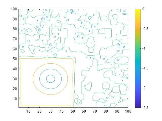
Create a matrix of data with one isolated valley and many valleys with high density elsewhere in the data.

rng("default")
data = zeros(100);
data(30,30) = 1000;
data = smoothdata2(data,"gaussian",50);
smallPeakLoc = randi(10000,1,400);
tempData = zeros(100)+1;
tempData(smallPeakLoc) = abs(randn(1,400))*3;
tempData(1:50,1:50) = 0;
A = -data-tempData;
A = smoothdata2(A,"gaussian",5);

contour(A)
colorbar

Figure contains an axes object. The axes object contains an object of type contour.

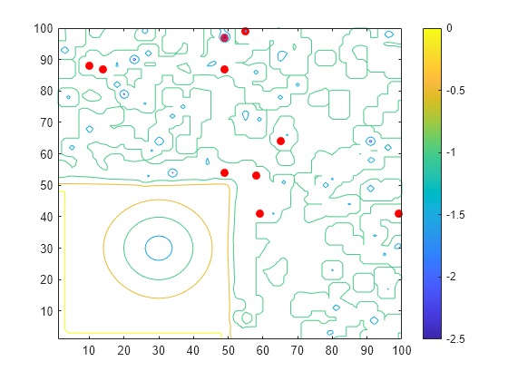
Because of the high density of valleys elsewhere in the data, islocalmin2 underestimates the prominence of the valley at (30,30).

TF = islocalmin2(A,MaxNumExtrema=10);
[X,Y] = meshgrid(1:100,1:100);

contour(A)
colorbar
hold on
plot3(X(TF),Y(TF),A(TF),"r.",MarkerSize=20)

Figure contains an axes object. The axes object contains 2 objects of type contour, line. One or more of the lines displays its values using only markers

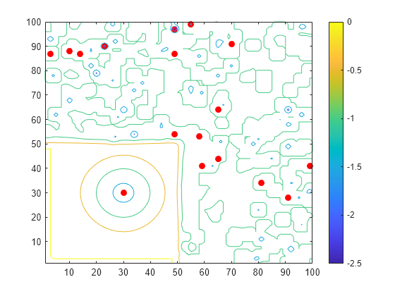
To limit the impact of distant valleys on the prominence calculation, specify a prominence window. The isolated valley at (30,30) is now marked as a local minima.

TF2 = islocalmin2(A,ProminenceWindow=50,MaxNumExtrema=10);
contour(A)
colorbar
hold on
plot3(X(TF2),Y(TF2),A(TF2),"r.",MarkerSize=20)

Figure contains an axes object. The axes object contains 4 objects of type contour, line. One or more of the lines displays its values using only markers

Input Arguments

collapse all

Input data, specified as a vector, matrix, or multidimensional array.

islocalmin2 ignores missing values when computing the local minima.

Name-Value Arguments

Specify optional pairs of arguments as Name1=Value1,...,NameN=ValueN, where Name is the argument name and Value is the corresponding value. Name-value arguments must appear after other arguments, but the order of the pairs does not matter.

Example: TF = islocalmin2(A,MinProminence=2)

Sample points, specified as a two-element cell array of vectors of sample point values. The sample points in the first vector represent the data locations along the columns of A, and the sample points in the second vector represent the data locations along the rows of A.

Both vectors must be sorted and must not contain duplicate elements. Sample points do not need to be uniformly spaced. If A is an m-by-n matrix, then the default value of SamplePoints is {1:n 1:m}.

The prominence window is defined relative to the sample points. When the sample point vectors have data type datetime or duration, the prominence window size must have type duration.

Example: islocalmin2(A,SamplePoints={1:5,10:2:18})

Minimum prominence, specified as a nonnegative scalar. islocalmin2 returns only local minima whose prominence is at least the specified value.

Prominence window size, specified as a positive integer or duration scalar, two-element cell array of positive integer or duration values, or two-element cell array of two-element vectors of nonnegative integer or duration values. islocalmin2 defines the window relative to the sample points.

  • If ProminenceWindow is a positive integer scalar k, then the window is a k-by-k block centered about the current element.

  • If ProminenceWindow is a two-element cell array of positive integers {m n}, then the window is an m-by-n block centered about the current element.

  • If ProminenceWindow is a two-element cell array of two-element vectors of nonnegative integers {[bRow fRow] [bCol fCol]}, then the window contains the row and column of the current element, the preceding bRow and succeeding fRow rows, and the preceding bCol and succeeding fCol columns.

If you specify SamplePoints using datetime or duration values, then ProminenceWindow must be of type duration.

Example: islocalmin2(A,ProminenceWindow=4)

Example: islocalmin2(A,ProminenceWindow={2 3})

Example: islocalmin2(A,ProminenceWindow={[0 2] [3 3]})

Flat region indicator for when a local minimum value is repeated in adjacent elements, specified as one of these values:

  • "center" — Select only the center (centroid) element of a flat region as the local minimum. "center" indicates exactly one local minimum per flat section.

  • "first" — Select only the first element of a flat region as the local minimum, where the first element is the element with the smallest linear index. "first" indicates exactly one local minimum per flat section and guarantees that all elements of TF with a value of 1 (true) are extrema.

  • "all" — Select all the elements of a flat region as the local minima. The number of elements of TF with a value of 1 (true) does not match the number of local minima.

When you specify the MinSeparation or MaxNumExtrema name-value argument, flat region points are jointly considered a single minimum point.

Minimum separation between local minima, specified as 0, a nonnegative integer or duration scalar, or a two-element cell array of positive integer or duration values.

If MinSeparation is a scalar, it is the Euclidean distance between minima. If MinSeparation is a cell array, the first element specifies the minimum distance between minima along the columns of A and the second element specifies the minimum distance along the rows of A. The separation values are defined in the same units as the sample points vectors, which are [1 2 3 ...] by default.

When the separation value is greater than 0, islocalmin2 selects the most prominent local minimum and ignores all other local minima within the specified separation. This process is repeated until there are no more local minima detected.

If you specify SamplePoints using datetime or duration values, the corresponding element in MinSeparation must be of type duration.

Example: islocalmin2(A,MinSeparation=3)

Example: islocalmin2(A,SamplePoints={1:10,hours(1:10)},MinSeparation={3,hours(4)})

Maximum number of minima to detect, specified as a positive integer scalar. islocalmin2 finds no more than the specified number of the most prominent minima.

Output Arguments

collapse all

Local minima indicator, returned as a vector, matrix, or multidimensional array. TF is the same size as A.

Data Types: logical

Prominence, returned as a vector, matrix, or multidimensional array. The prominence of a local minimum (or valley) measures how the valley stands out with respect to its depth and location relative to other valleys. For more information about the prominence calculation, see Algorithms.

P is the same size as A. If the input data has a signed or unsigned integer type, then P contains unsigned integers.

Algorithms

islocalmin2 identifies all local minima in the input data and follows these steps to compute the prominence of each local minimum:

  1. Determine the data to use to compute the prominence.

    • If the ProminenceWindow name-value argument is specified, use its value to draw a rectangular window of data around the current local minimum. Otherwise, use a rectangular window that includes all of the data.

  2. Determine the prominence box.

    • Move vertical lines left and right from the current minimum until encountering a lower minimum or the edge of the rectangular window.

    • Move horizontal lines up and down from the current minimum until encountering a lower minimum or the edge of the rectangular window.

  3. Compute the prominence.

    • Divide the prominence box into four quadrants centered on the current local minimum.

    • Identify the highest value within each quadrant.

    • Use the lowest of these quadrant maximum values as the basis value. The prominence is the absolute difference between the height of the current local minimum and the basis value.
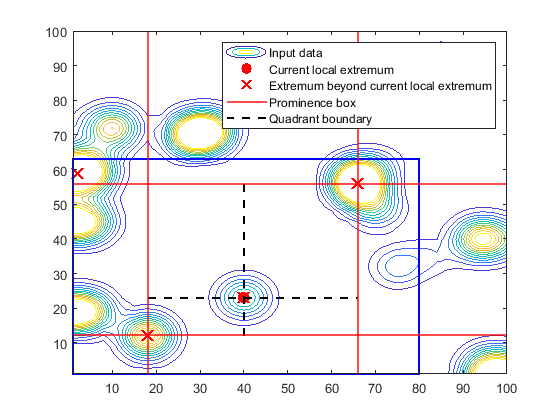
Contour plot of data with peaks. A rectangular window and a prominence box surround the current extremum. The prominence box is divided into four quadrants.

Version History

Introduced in R2024a

Go to top of page