Optimize Multi-Injection Diesel Engine Calibration Using Statistical Models
After creating the statistical models to fit the data, you can use them in optimizations. You can use the accurate statistical engine model to replace the high-fidelity simulation and run much faster, enabling the optimization to generate calibrations in feasible times.
Run an optimization to choose whether to use Pilot Injection at each operating point.
Optimize fuel consumption over the drive cycle, and meet these constraints:
Constrain total NOx
Constrain turbocharger speed
Constrain smoothness of tables
Fill lookup tables for all control inputs.
Set Up Models and Tables for Optimization
To perform an optimization, you need to import the statistical models created earlier in the Model Browser.
In MATLAB®, on the Apps tab, in the Automotive group, click MBC Optimization.
To see how to import models, on the home page, click Import From Project.
The CAGE Import Tool opens. Here, you can select models to import from a model browser project file or direct from the Model Browser if it is open. However, the toolbox provides an example file with the models already imported, so click Close to close the CAGE Import Tool.
On the home page, in the Case Studies list, select the multi-injection example, or select File > Open Project and browse to the example file
CI_MultiInject.cag, found inmatlab\toolbox\mbc\mbctraining.Click Models in the left Data Objects pane to view the models.
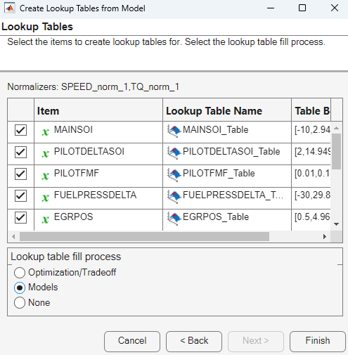
To see how to set up tables to fill with the results of your optimizations, select Tools > Create Lookup Tables from Model. The Create Lookup Tables from Model wizard opens.

Select the model BSFC and the Create operating point data set check box, and click Next.
If you left the defaults, you would use the model operating points for the table breakpoints. However, you need to create different tables to the operating points.
Clear the Use model operating points check box.
Select
SPEEDandTQfor the axis inputs.Enter
11for the table rows and columns.
Click Next.
View the last screen to see how many tables CAGE will create for you if you finish the wizard.
Click Cancel to avoid creating new unnecessary tables in your example file. The example file already contains all the tables needed for your calibration results.
Select the Lookup Tables view to see all the tables. Observe there are tables named
_wPilotand_noPilotthat will be filled by optimization results. The goal is to fill separate tables for each mode, pilot injection active and no pilot injection.
Examine the Point Optimization Setup
The example file CI_MultiInject.cag shows the results of the multistage
process to finish this calibration.
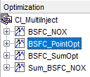
Click Optimization in the left Processes pane to view the optimizations.
To complete the calibration, you need to start with a point optimization to determine whether to use Pilot Injection at each operating point. You use the results of this point optimization to set up the sum optimization to optimize fuel consumption over the drive cycle, and meet these constraints:
Constrain total NOx
Constrain turbocharger speed
Constrain smoothness of tables
Select the
BSFC_PointOptoptimization to view the setup.View the two objectives in the Objectives pane. These are set up to minimize
BSFCandPEAKPRESS. Double-click an objective to view its settings.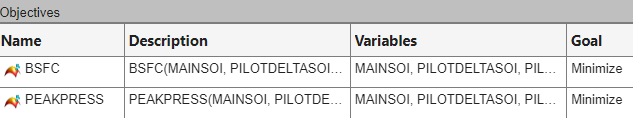
Observe that the Constraints pane shows a boundary model constraint.
Learn the easiest way to set up an optimization like this by selecting Tools > Create Optimization from Model.
In the Optimization Quick Start dialog box:
On the Objectives page:
Set Optimization type to
Modal optimization: find
              optimal operating mode (requires composite models)
. The optimization identifies which pilot mode (active pilot injection or no pilot injection) is best to use at each operating point.Set Model to
BSFC.Set Goal to
minimize.

Click Next.
The optimization is constrained by a model boundary constraint. Click Next again.
The optimization specifies Operating points as
Unique
        operating points
. Click Apply to create the optimization.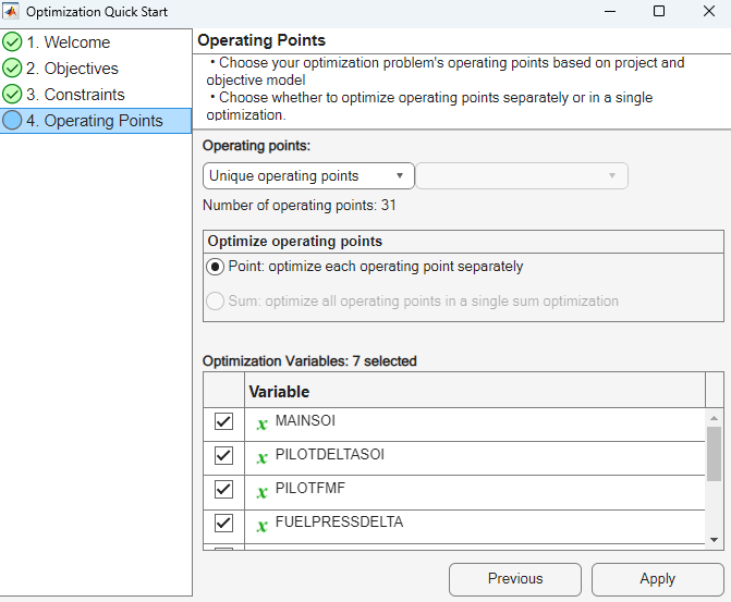
Compare your new optimization with the example
BSFC_PointOpt. Notice the example has a second objective, to minimizePEAKPRESS. To see how to set this up, right-click the Objectives pane and select Add Objective.
Examine the Point Optimization Results
The example file CI_MultiInject.cag shows the results of the multistage
process to finish this calibration.
Expand the first optimization node,
BSFC_PointOpt, and select the output node underneath,BSFC_PointOpt_Output.Select View > Selected Solution (or the toolbar button) to view which mode the optimization selected as best at each operating point. The left-hand pane provides all optimization results. The right-hand pane provides the results for the current run.
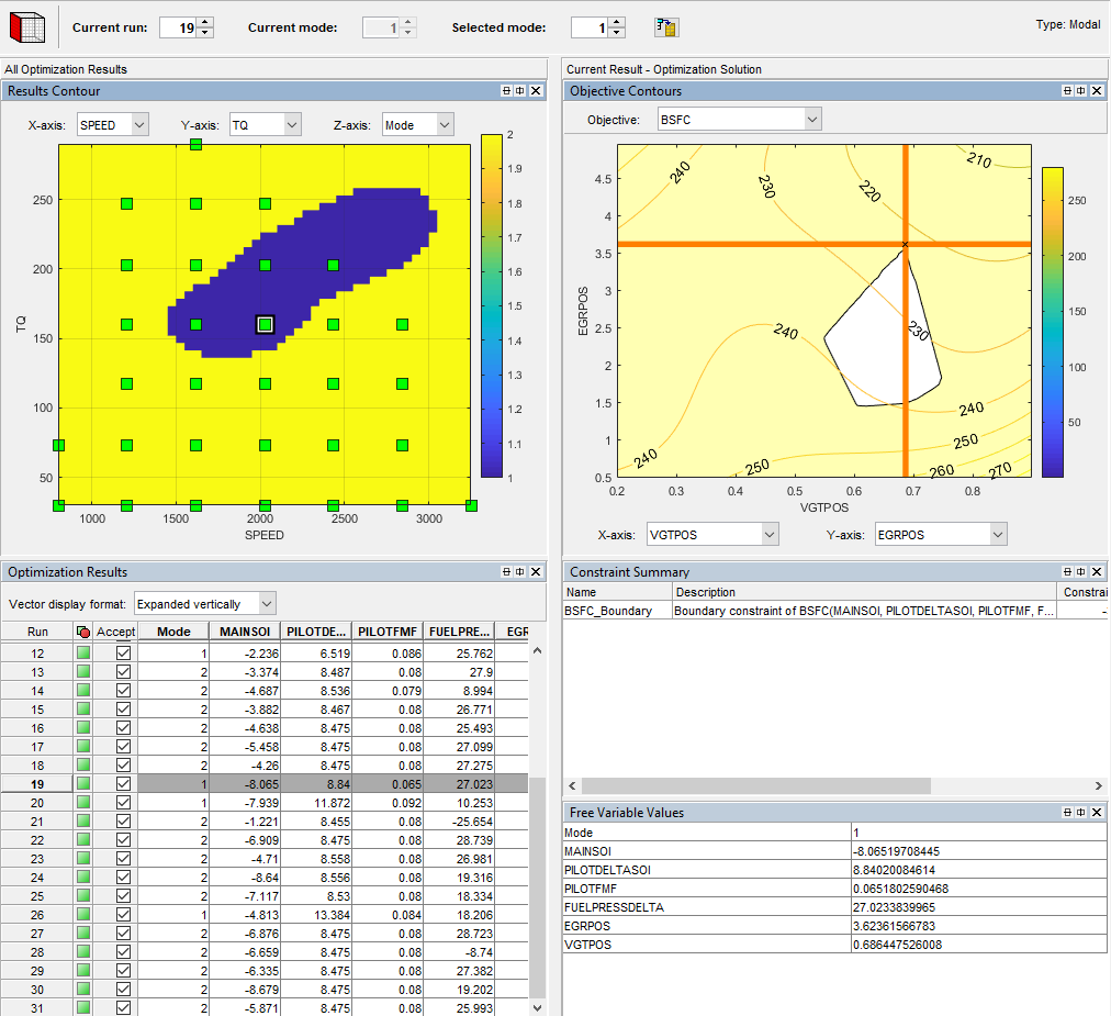
Review the Results Contour plot to see which mode has been selected across all operating points. Use this view to verify the distribution of mode selection.
Click to select a point in the table or Results Contour, and you can use the Selected solution controls at the top to alter which mode is selected at that point. You might want to change selected mode if another mode is also feasible at that point. For example, you can change the mode to make the table more smooth.
Use the other objectives to explore the results. For example, you might want to manually change the selected mode based on an extra objective value. It can be useful to view plots of the other objective values at your selected solutions. To display another plot or change the view, right-click the plots to view the options.
For example, right-click the Objective Contours plot. Select Current View > Objective Graphs.
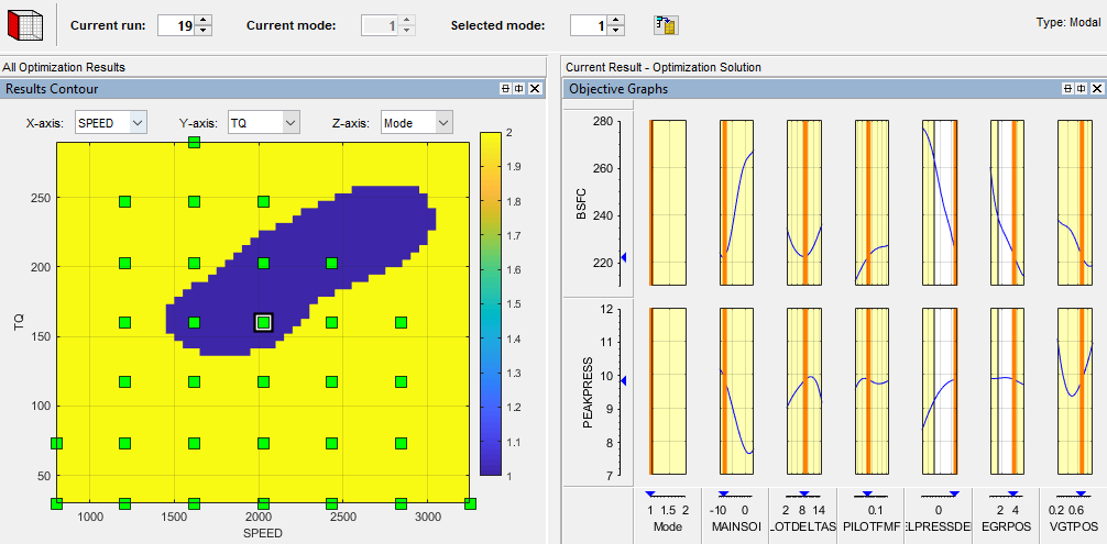
To see both solutions for a particular operating point, use the Pareto Slice view. You can inspect the objective value (and any extra objective values) for each solution. If needed, you can manually change the selected mode to meet other criteria, such as the mode in adjacent operating points, or the value of an extra objective.
For details on tools for choosing a mode at each operating point, see Analyze Modal Optimization Results.
Create Sum Optimization from Point Optimization
The point optimization results determine whether to use pilot injection at each operating point. When you are satisfied with all selected solutions for your modal optimization, you can make a sum optimization over all operating points. The pilot injection mode must be fixed in the sum optimization to avoid optimizing too many combinations of operating modes.
The results of the point optimization were used to set up the sum optimization to optimize fuel consumption over the drive cycle. To see how to do this:
From the point optimization output node,
BSFC_PointOpt_Output, select Solution > Create Sum Optimization.The toolbox automatically creates a sum optimization for you with your selected best mode for each operating point. The create sum optimization function converts the modal optimization to a standard single objective optimization (
fminconalgorithm) and changes theMode Variableto a fixed variable.Compare your new optimization with the example sum optimization,
BSFC_SumOpt. The example shows you need to set up more constraints to complete the calibration.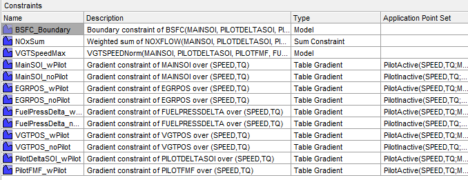
The additional constraints make the optimization meet these requirements:
Constrain total NOx
Constrain maximum turbocharger speed
Constrain smoothness of tables with gradient constraints
Import all required constraints to your new optimization by selecting Optimization > Constraints > Import Constraints. Select the example sum optimization and import all but the first boundary model constraint.
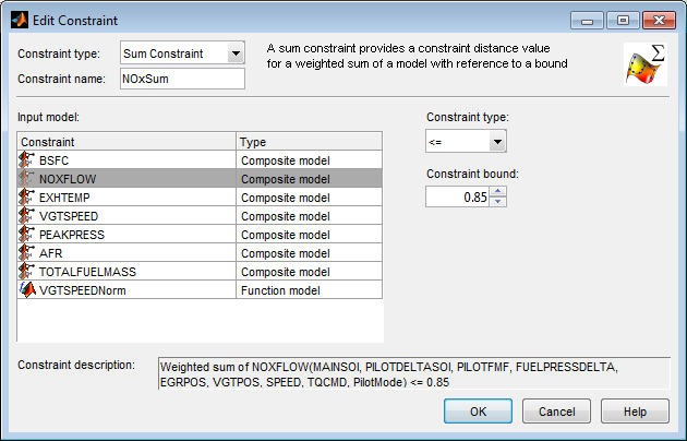
Double-click the additional constraints to open the Edit Constraint dialog box and view the setup.
This sum constraint controls the total NOx.
This constraint controls maximum turbocharger speed.
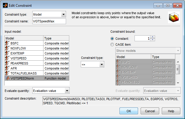
Observe that this constraint does not use the
VGTSPEEDmodel directly, but instead uses a function modelVGTSPEEDNorm. You can examine this function model in the Models view. The function model scales the constraint to help the optimization routines, which have problems if constraints have very different sizes.VGTSPEEDis of order of165000, while the other constraints are of the order of 1, so the function modelVGTSPEEDNormnormalizesVGTSPEEDby dividing it by165000.The following constraint controls the gradient across the
MAINSOItable.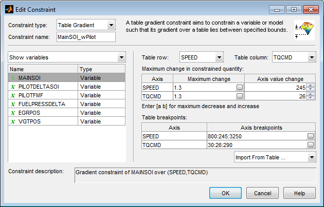
In the Optimization view, in the Constraints pane, observe that:
The gradient constraints are in pairs, one with pilot and one with no pilot. Separate table gradient constraints are required for different modes because the goal is to fill separate tables for each mode.
All the gradient constraints have an entry in the Application Point Set column.
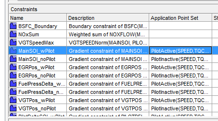
Right-click the table gradient constraint
MainSOI_wPilotand click Select Application Point Set to see how these are set up.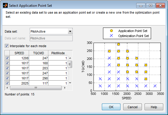
Observe the Interpolate for each mode option is selected. This application point set restricts the table gradient constraint to
Mode1 (active) points only. You can create an application point set like this by selectingNew subsetand then choosing a subset of the optimization points by clicking in the plot or table. The application points here correspond to the operating points where the point optimization determined that the pilot mode should be active (Mode= 1). For comparison, here is the results contour plot for the point optimization results.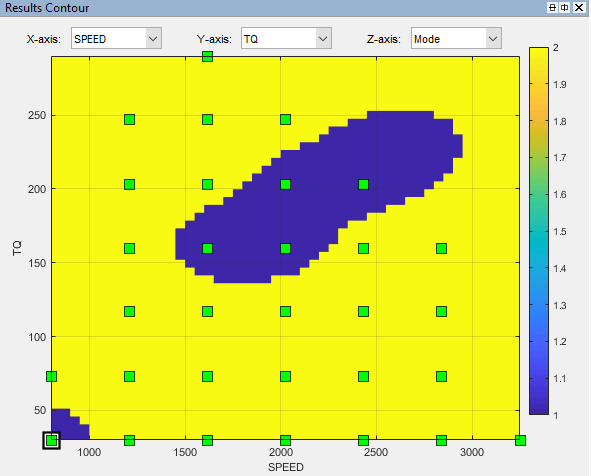
Compare the results contour plot with the application points for the next table gradient constraint,
MainSOI_noPilot. These application points restrict the table gradient constraint toMode2 points only, where the pilot is inactive.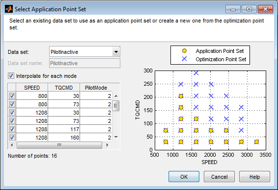
Your sum optimization now contains all the required constraints and is ready to run. Next, view the results in the example sum optimization.
Fill Lookup Tables from Optimization Results
CAGE remembers lookup table filling settings. To view how the example tables are filled:
Expand the example sum optimization node
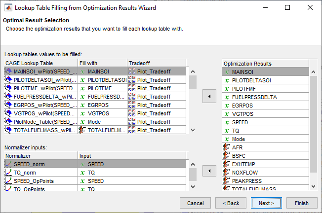
BSFC_SumOptand select theBSFC_SumOpt_Outputnode.Select Solution > Fill Lookup Tables (or use the toolbar button) to open the Lookup Table Filling from Optimization Results Wizard.
On the first screen, observe all the tables in the CAGE tables to be filled list. Click Next.
On the second screen, observe all the tables are matched up with optimization results to fill them with. Click Next.
On the third screen, observe how some tables have a Filter Rule set up so that they are filled only with results where
Modeis 1 or 2. You can create a filter rule like this by enteringMode==1in the Filter Rule column.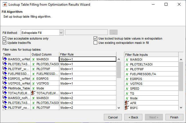
You can either click Finish to fill all the tables, or Cancel to leave the tables untouched. The example tables are already filled with these settings.
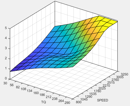
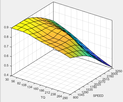
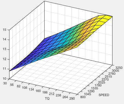
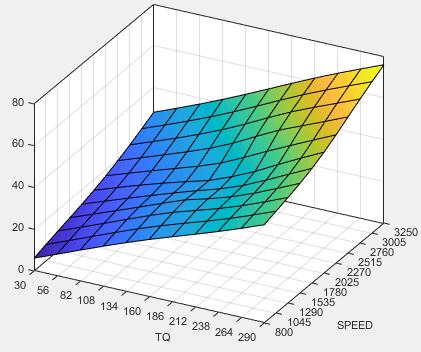
These plots show results similar to the calibration results.
Pilot Mode Table
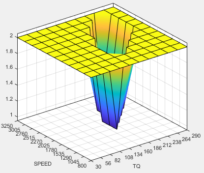
You need to fill calibration tables for each control variable described in Multi-Injection Diesel Problem Definition, in both pilot modes, active and inactive.
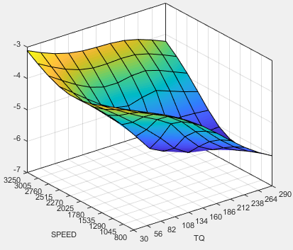
Following are all the pilot active tables.
Main Injection Timing (SOI) Table
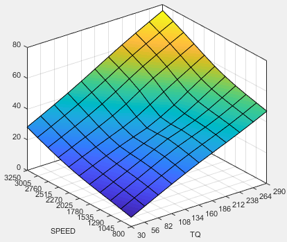
Total Injected Fuel Mass Table
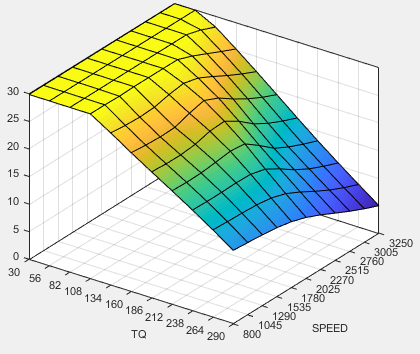
Fuel Pressure Delta Table
Exhaust Gas Recirculation (EGR) Valve Position Table
Variable-Geometry Turbo (VGT) Position Table
Pilot Injection Timing (Pilot SOI Delta) Table
Pilot Fuel Mass Fraction Table
Examine the Multiobjective Optimization
The example file CI_MultiInject.cag also shows an example multiobjective
optimization. This can useful for calibrations where you want to minimize more than one
objective at a time, in this case, BSFC and NOX. The
multiobjective optimization uses the gamultiobj algorithm.
Select the
BSFC_NOXnode to see how the optimization is set up. Observe the 2 objectives and the optimization information: Multiobjective optimization using a genetic algorithm.Expand the
BSFC_NOXnode and select theBSFC_NOX_Outputto view the results. To select the view that you want to examine, right-click in the pane and select Current View. Select the view.Examine the Pareto graphs. It can be useful to display the Solution Information view at the same time to view information about a selected solution. You might want to select a dominated solution (orange triangle) over a pareto solution (green square) to trade off desired properties.

Select the
Sum_BSFC_NOXnode to see how the sum optimization is set up. The sum optimization was created from the point optimization results. Observe the 2 objectives and all the constraints.Expand the
Sum_BSFC_NOXnode and select theSum_BSFC_NOX_Outputto view the results.
Tip
Learn how MathWorks® Consulting helps customers develop engine calibrations that optimally balance engine performance, fuel economy, and emissions requirements: see Optimal Engine Calibration.