Create an Optimal Design
Optimal designs are best for cases with high system knowledge, where previous studies have given confidence on the best type of model to be fitted, and the constraints of the system are well understood. Optimal designs require linear models.
Click the
 button in the toolbar or select File > New Design. A new node appears in the design tree. It is named
according to the model for which you are designing, for example,
button in the toolbar or select File > New Design. A new node appears in the design tree. It is named
according to the model for which you are designing, for example,
Linear Model Design.Select the node in the tree by clicking. An empty Design Table appears if you have not yet chosen a design. Otherwise, if this is a new child node the display remains the same, because child nodes inherit all the parent design's properties.
Set up any constraints at this point. See Define Design Constraints.
Choose an Optimal design by clicking the
 button in the toolbar, or choose Design > Optimal.
The optimal designs in the Design Editor are formed using the following process:
An initial starting design is chosen at random from a set of defined candidate points.
p additional points are added to the design, either optimally or at random. These points are chosen from the candidate set.
p points are deleted from the design, either optimally or at random.
If the resulting design is better than the original, it is kept.
This process is repeated until either (a) the maximum number of iterations is exceeded or (b) a certain number of iterations has occurred without an appreciable change in the optimality value for the design.
The Optimal Design dialog box consists of three tabs that contain the settings for three main aspects of the design:
Initial Design tab: Starting point and number of points in the design
Candidate Set tab: Candidate set of points from which the design points are chosen
Algorithm tab: Options for the algorithm that is used to generate the points
Optimal Design: Initial Design Tab
The Initial Design tab allows you to define the composition of the initial design: how many points to keep from the current design and how many total or additional points to choose from the candidate set.
Choose the type of the optimal design, using the Optimality criteria drop-down menu:
D-Optimaldesigns — Aims to reduce the volume of the confidence ellipsoid to obtain accurate coefficients. This is set up as a maximization problem, so the progress graph should go up with time.The D-optimality value used is calculated using the formula
 where X is the regression
matrix and k is the number of terms in the
regression matrix.
where X is the regression
matrix and k is the number of terms in the
regression matrix.V-Optimaldesigns — Minimizes the average prediction error variance, to obtain accurate predictions. This is better for calibration modeling problems. This is a minimization process, so the progress graph should go down with time.The V-optimality value is calculated using the formula
where xj are rows in the regression matrix, XC is the regression matrix for all candidate set points, and nC is the number of candidate set points.
A-Optimaldesigns — Minimizes the average variance of the parameters and reduces the asphericity of the confidence ellipsoid. The progress graph also goes down with this style of optimal design.The A-optimality value is calculated using the formula
where X is the regression matrix.
You might already have points in the design (if the new design node is a child node, it inherits all the properties of the parent design). If so, choose from the radio buttons:
Replace the current points with a new initial design
Augment the current design with additional points
Keep only the fixed points from the current design
For information on fixed design points, see Fixing, Deleting, and Sorting Design Points.
You can choose the total number of points and/or the number of additional points to add by clicking the up/down buttons or by typing directly into the edit boxes for Optional additional points or Total number of points.
Optimal Design: Candidate Set Tab
The Candidate Set tab allows you to set up a candidate set of points for your optimal design. Candidate sets are a set of potential test points. This typically ranges from a few hundred points to several hundred thousand.
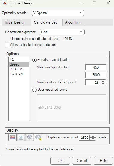
The set generation schemes are as follows:
Grid— Full factorial grids of points, with fully customizable levels.Grid/Lattice— A hybrid set where the main factors are used to generate a lattice, which is then replicated over a small number of levels for the remaining factors.Halton Sequence— Halton Sequence designs are generated from thehaltonsetclass in the Statistics and Machine Learning Toolbox™ software. See Halton Sequence for more informationLattice— These have the same definition as the space-filling design lattices, but are typically used with about 10,000 points. The advantage of a lattice is that the number of points does not increase as the number of factors increases; however, you do have to try different prime number generators to achieve a good lattice. See Lattice.Sobol Sequence— Sobol sequence designs are generated from thesobolsetclass in the Statistics and Machine Learning Toolbox software. See Sobol Sequence for more information.Stratified Lattice— Another method of using a lattice when some factors cannot be set to arbitrary values. Stratified lattices ensure that the required number of levels is present for the chosen factor. Note that you cannot set more than one factor to stratify to the same N levels. This is because forcing the same number of levels would also force the factors to have the same generator. As for a lattice space-filling design, no two factors can have the same generator, because in such cases the lattice points all fall on the main diagonal of that particular pairwise projection, creating highly visible planes in the points and poor coverage of the space. For illustrations of this effect, see Lattice.User-defined— Import custom matrices of points from MATLAB® software or MAT-files.
For each factor you can define the range and number of different levels within that range to select points.
Choose a type of generation algorithm from the drop-down menu. Note that you could choose different parameters for different factors (within an overall scheme such as
Grid).This tab also has buttons for creating plots of the candidate sets. Try them to preview your candidate set settings. If you have created a custom candidate set you can check it here. The edit box sets the maximum number of points that will be plotted in the preview windows. Candidate sets with many factors can quickly become very large, and attempting to display the entire set will take too long. If the candidate set has more points than you set as a maximum, only every
Nth point is displayed, whereNis chosen such that (a) the total displayed is less than the maximum and (b)Nis prime. If you think that the candidate set preview is not displaying an adequate representation of your settings, try increasing the maximum number of points displayed.Notice that you can see 1D, 2D, 3D, and 4D displays (fourth factor is color) all at the same time as they appear in separate windows (see the example following). Move the display windows (click and drag the title bars) so you can see them while changing the number of levels for the different factors.
You can change the factor ranges and the number of levels using the edit boxes or buttons.
Optimal Design: Algorithm Tab
The Algorithm tab has the following algorithm details:
Augmentation method —
RandomorOptimal— Optimal can be very slow (searches the entire candidate set for points) but converges using fewer iterations. Random is much faster per iteration, but requires a larger number of iterations. The Random setting does also have the ability to lower the optimal criteria further when the Optimal setting has found a local minimum.Deletion method —
RandomorOptimal— Optimal deletion is much faster than augmentation, because only the design points are searched.p — number of points to alter per iteration — The number of points added/removed per iteration. For optimal augmentation this is best kept smaller (~5); for optimal deletion only it is best to set it larger.
Delta — value below which the change in optimality criteria triggers an increment in q — This is the size of change below which changes in the optimality criteria are considered to be not significant.
q — number of consecutive non-productive iterations which trigger a stop — Number of consecutive iterations to allow that do not increase the optimality of the design. This only has an effect if random augmentation or deletion is chosen.
Maximum number of iterations to perform — Overall maximum number of iterations.
Choose the augmentation and deletion methods from the drop-down menus (or leave at the defaults).
You can alter the other parameters by using the buttons or typing directly in the edit boxes.
Click OK to start optimizing the design.
When you click the OK button on the Optimal Design dialog box, another window appears that contains a graph. This window shows the progress of the optimization and has two buttons: Accept and Cancel. Accept stops the optimization early and takes the current design from it. Cancel stops the optimization and reverts to the original design.
You can click Accept at any time, but it is most useful to wait until iterations are not producing noticeable improvements; that is, the graph becomes very flat.
You can always return to the Optimal Design dialog box (following the same steps) and choose to keep the current points while adding more.
Averaging Optimality Across Multiple Models
The Design Editor can average optimality across several linear models. This is a flexible way to design experiments using optimal designs. If you have no idea what model you are going to fit, you would choose a space-filling design. However, if you have some idea what to expect, but are not sure which model to use, you can specify a number of possible models. The Design Editor can average an optimal design across each model.
For example, if you expect a quadratic and cubic for three factors but are unsure about a third, you can specify several alternative polynomials. You can change the weighting of each model as you want (for example, 0.5 each for two models you think equally likely). This weighting is then taken into account in the optimization process in the Design Editor. See Global Model Class: Multiple Linear Models.