Manipulate Designs
Adding and Editing Design Points
Adding Design Points
In any design, you can add points by selecting Edit > Add Point. You can choose how to add points: extend a space-filling sequence (for space-filling designs), optimally (for optimal designs), randomly, or at specified values. For space-filling designs, when you want to collect more data, you can add design points that continue the same space-filling sequence in your original design. This allows you to collect more data filling in the gaps between your previous design points. You can progressively augment Halton and Sobol sequence space-filling designs to add points with the same sequence parameters. You can add points to your original space-filling sequence, preserving the original points and adding new ones with the same sequence parameters.
Tip
In case you want to add more points later, to preserve the
space-filling sequence of a design, copy the design before
constraining or editing the design. If you do not create a copy
of the design, when you edit, you lose the original
space-filling settings and then you cannot extend the sequence.
When design type changes to Custom, you
cannot access the original sequence settings to add new
points.
To preserve your original design when you add new points, create a child design of your original unconstrained design. Select your design, and click the New Design
 button in the
toolbar, or select File > New.
button in the
toolbar, or select File > New.The new child design, identical to the parent, is selected in the tree.
To add space-filling, optimal, custom, or random points, select Edit > Add Point or click the
 button. A dialog box
appears, as shown following.
button. A dialog box
appears, as shown following.Choose an augmentation method from the drop-down menu. Options depend on your design type and include: extend sobol or halton sequence, optimal (D,V, or A), random, or user-specified.
Note
You can add points optimally to any design based on a linear or multilinear model, as long as it has the minimum number of points required to fit that model. This means that after adding a constraint you might remove so many points that a subsequent replace operation does not allow optimal addition.
For space-filling designs, use
Extend Sobol SequenceorExtend Halton Sequenceto preserve the original points and add new ones with the same sequence parameters.Choose the number of points to add, using the buttons or typing into the edit box. For space-filling designs, observe the new points on the plot.
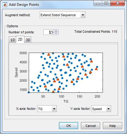
For user-specified custom points, enter the values of each factor for each point you want to add.
If you choose an optimal augmentation method and click Edit, the Candidate Set dialog box appears. Edit the ranges and levels of each factor and which generation algorithm to use. These are the same controls you see on the Candidate Set tab of the Optimal Design dialog box. Click OK.
Click OK to add the new points and close the Add Design Points dialog box.
In the Design Editor, for space-filling designs, these steps can be helpful:
Use the pairwise view, switching between the parent and child designs to visually verify that the new points have been added while preserving your original points.
Create a copy child design to add constraints. Preserving your unconstrained parent design allows you to add more points later if you need to. See also Space-Filling Design Augmentation Restrictions.
New points are added to the end of the list of existing points. If you want to extract only the augmented points for testing, select Edit > Delete Point to open a dialog box in which you can choose the points to delete. See Fixing, Deleting, and Sorting Design Points.
Round and sort your data before sending it out for testing. Select Edit > Round Factor to limit decimal places of factors. Select Edit > Sort to sort the points for test efficiency, because operators often test in order of speed followed by load. See Fixing, Deleting, and Sorting Design Points.
Editing Design Points
Tip
In case you want to add more points later, to preserve the
space-filling sequence of a design, copy the design before
editing points. If you do not create a copy of the design, when
you edit points, you lose the original space-filling settings
and then you cannot extend the sequence. When design type
changes to Custom, you cannot access the
original sequence settings to add new points.
To edit particular points,
Right-click the title bar of one of the Design Editor views and select Current View > Design Table to change to the Table view. This gives a numbered list of every point in the design, so you can see where points are in the design.
To edit points, click to select table cells and type new values. You can also right-click table cells and select Copy or Paste. You can click and drag to select multiple cells to copy or paste.
Merging Designs
You can merge the points from two or more designs together using the File menu. You can merge designs together to form a new design, or merge points into one of the chosen designs. Points that are merged retain their fixed status in the new design.
Select File > Merge Designs. A dialog box appears, as shown.
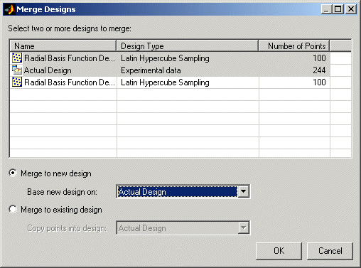
A list of all the designs from the Design Editor is shown, along with the associated design style and number of points. Select two or more designs from the list by dragging with the mouse or Ctrl+clicking.
When at least two designs have been selected, the options at the bottom of the dialog box are enabled. Choose whether you want to create a new design or put the design points into an existing design.
If you choose to create a new design, you must also choose one of the selected designs to act as a base. Properties such as the model, constraints, and any optimal design setup are copied from this base design. If you choose to reuse an existing design you must choose one of the selected designs to receive the points from other designs.
Click OK to perform the merging process and return to the main display. If you choose to create a new design, it appears at the end of the design tree.
Fixing, Deleting, and Sorting Design Points
You can fix or delete points using the Edit menu. You can also sort points or clear all points from the design.
Tip
In case you want to add more points later, to preserve the
space-filling sequence of a design, copy the design before editing,
rounding, or sorting points. If you do not create a copy of the
design, when you edit points, you lose the original space-filling
settings and then you cannot extend the sequence. When design type
changes to Custom, you cannot access the original
sequence settings to add new points.
Fixed points become red in the main Design Editor table display. If you have matched data to a design or used experimental data as design points, those points are automatically fixed. You already have the data points, so you do not want them to be changed or deleted. Design points that have been matched to collected data are also fixed. Since these points have already been run they cannot be freed — you will not see them in the Fix Design Points dialog box. Once you have fixed points, they are not moved by design optimization processes. This automatic fixing makes it easy for you to optimally augment the fixed design points.
To fix or delete points:
To delete all points in the current design, select Edit > Clear.
If you want to fix or delete particular points, first change a Design Editor display pane to the Table view. This gives a numbered list of every point in the design, so you can see where points are in the design.
Select Edit > Fix/Free Points or Edit > Delete Point (or click the toolbar button
 ).
).A dialog box appears in which you can choose the points to fix or delete.
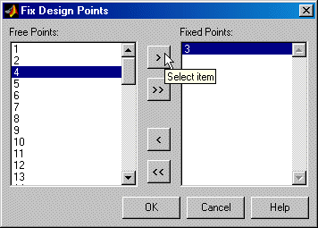
The example above shows the dialog box for fixing or freeing points. The dialog box for deleting points has the same controls for moving points between the Keep Points list and the Delete Points list.
Move points from the Free Points list to the Fixed Points list; or from the Keep Points list to the Delete Points list, by using the buttons.
Click OK to complete the changes specified in the list boxes, or click Cancel to return to the unchanged design.
To sort points:
Select Edit > Sort. A dialog box appears (see example following) for sorting the current design — by ascending or descending factor values, randomly, or by a custom expression.
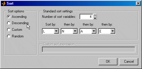
To sort by custom expression you can use MATLAB® expressions (such as
abs(N)for the absolute value ofN) using the input symbols. Note that sorts are made using coded units (from -1 to 1) so remember that points in the center of your design space will be near zero in coded units, and those near the edge will tend to 1 or -1.Select Edit > Randomize as a quick way of randomly resorting the points in the current design. This is a shortcut to the same functionality provided by the Random option in the Sort dialog box.
Prediction Error Variance Viewer
Introducing the Prediction Error Variance Viewer
You can use the Prediction Error Variance (PEV) viewer to examine the quality of the model predictions. You can examine the properties of designs or global models. When you open it from the Design Editor, you can see how well the underlying model predicts over the design region. When you open it from a global model, you can view how well the current global model predicts. A low PEV (tending to zero) means that good predictions are obtained at that point.
The Prediction Error Variance Viewer is only available for linear models and radial basis functions.
When designs are rank deficient, the Prediction Error Variance Viewer appears but is empty; that is, the PEV values cannot be evaluated because there are not enough points to fit the model.
From the Design Editor, select Tools > Prediction Error Variance Viewer.
From the global level of the Model Browser, if the selected global model is linear or a radial basis function,
Click the
 toolbar button to
open the Prediction Error Variance Viewer.
toolbar button to
open the Prediction Error Variance Viewer.Alternatively, select Model > Utilities > Prediction Error Variance Viewer.
If a model has child nodes you can only select the Prediction Error Variance Viewer from the child models.
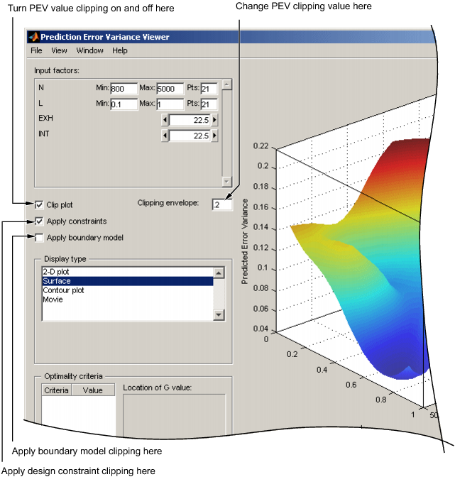
The default view is a 3D plot of the PEV surface.
The plot shows where the model predictions are best. The model predicts well where the PEV values are lowest.
If you have transformed the output data (e.g. using a Box-Cox transform), then the Prediction Error Variance Viewer displays the predicted variance of the transformed model.
Display Options
The View menu has many options to change the look of the plots.
You can change the factors displayed in the 2D and 3D plots. The drop-down menus below the plot select the factors, while the unselected factors are held constant. You can change the values of the unselected factors using the buttons or edit boxes in the frame, top left.
The
Movieoption shows a sequence of surface plots as a third input factor's value is changed. You can change the factors, replay, and change the frame rate.You can change the number, position, and color of the contours on the contour plot with the Contours button. See the contour plot section (in Response Surface View) for a description of the controls.
You can select the Clip Plot check box, as shown in the preceding example. Areas that move above the PEV value in the Clipping envelope edit box are removed. You can enter the value for the clipping envelope. If you do not select Clip Plot, a white contour line is shown on the plot where the PEV values pass through the clipping value.
You can also clip with the boundary model or design constraints if available. Select the check boxes Apply constraint or Apply boundary model to clip the plot.
When you use the Prediction Error Variance Viewer to see design properties, optimality values for the design appear in the Optimality criteria frame.
Note that you can choose Prediction Error shading in the Response Feature view (in Model Selection or Model Evaluation). This shades the model surface according to Prediction Error values (sqrt(PEV)). This is not the same as the Prediction Error Variance Viewer, which shows the shape of a surface defined by the PEV values. See Response Surface View.
Optimality Criteria. No optimality values appear in the Optimality criteria frame until you click Calculate. Clicking Calculate opens the Optimality Calculations dialog box. Here iterations of the optimization process are displayed.
In the Optimality criteria frame in the Prediction Error Variance Viewer are listed the D, V, G and A optimality criteria values, and the values of the input factors at the point of maximum PEV (Location of G value). This is the point where the model has its maximum PEV value, which is the G-optimality criteria. The D, V and A values are functions of the entire design space and do not have a corresponding point.
For statistical information about how PEV is calculated, see the next section Prediction Error Variance.
Prediction Error Variance
Prediction Error Variance (PEV) is a very useful way to investigate the predictive capability of your model. It gives a measure of the precision of a model's predictions.
You can examine PEV for designs and for models. It is useful to remember that:
PEV (model) = PEV (design) * MSE
So the accuracy of your model's predictions is dependent on the design PEV and the mean square errors in the data. You should try to make PEV for your design as low as possible, as it is multiplied by the error on your model to give the overall PEV for your model. A low PEV (close to zero) means that good predictions are obtained at that point.
You can think of the design PEV as multiplying the errors in the data. If the design PEV < 1, then the errors are reduced by the model fitting process. If design PEV >1, then any errors in the data measurements are multiplied. Overall the predictive power of the model will be more accurate if PEV is closer to zero.
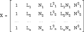
You start with the regression (or design) matrix, for example, for a quadratic in N (engine speed) and L (load or relative air charge):
If you knew the actual model, you would know the actual model
coefficients ![]() . In this case the observations would be:
. In this case the observations would be:
![]()
where ![]() is the measurement error with
variance
is the measurement error with
variance
![]()
However you can only ever know the predicted coefficients:
![]()
which have variance
![]()
Let x be the regression matrix for some new point where you want to evaluate the model, for example:
![]()
Then the model prediction for this point is:
![]()
Now you can calculate PEV as follows:
![]()
![]()
Note the only dependence on the observed values is in the variance (MSE) of the measurement error. You can look at the PEV(x) for a design (without MSE, as you don't yet have any observations) and see what effect it will have on the measurement error - if it is greater than 1 it will magnify the error, and the closer it is to 0 the more it will reduce the error.
You can examine PEV for designs or global models using the Prediction Error Variance viewer. When you open it from the Design Editor, you can see how well the underlying model predicts over the design region. When you open it from a global model, you can view how well the current global model predicts. A low PEV (tending to zero) means that good predictions are obtained at that point. See Prediction Error Variance Viewer.
For information on the calculation of PEV for two-stage models, see Prediction Error Variance for Two-Stage Models.
Prediction Error Variance for Two-Stage Models
It is very useful to evaluate a measure of the precision of the model's predictions. You can do this by looking at Prediction Error Variance (PEV). Prediction error variance will tend to grow rapidly in areas outside the original design space. The following section describes how PEV is calculated for two-stage models.
For linear global models applying the variance operator to Equation 15 yields:
![]() so
so
| (1) |
since Var(P) = W. Assume that it is required to calculate both the response features and their associated prediction error variance for the ith test. the predicted response features are given by:
| (2) |
where ![]() is an appropriate global covariate matrix.
Applying the variance operator to Equation 2
yields:
is an appropriate global covariate matrix.
Applying the variance operator to Equation 2
yields:
| (3) |
In general, the response features are non-linear functions of the
local fit coefficients. Let ![]() denote the non-linear function mapping
denote the non-linear function mapping
![]() onto
onto ![]() . Similarly let
. Similarly let ![]() denote the inverse mapping.
denote the inverse mapping.
| (4) |
Approximating ![]() using a first order Taylor series expanded about
using a first order Taylor series expanded about
![]() (the true and unknown fixed population value) and
after applying the variance operator to the result:
(the true and unknown fixed population value) and
after applying the variance operator to the result:
| (5) |
where the dot notation denotes the Jacobian matrix with respect to the
response features, ![]() . This implies that
. This implies that ![]() is of dimension (pxp). Finally the predicted
response values are calculated from:
is of dimension (pxp). Finally the predicted
response values are calculated from:
| (6) |
Again, after approximating f by a first order
Taylor series and applying the variance operator to the result:
| (7) |
After substituting Equation 3 into Equation 7 the desired result is obtained:
| (8) |
This equation gives the value of Prediction Error Variance.
Design Evaluation Tool
Introducing the Design Evaluation Tool
The Design Evaluation tool is only available for linear models.
You can open the Design Evaluation tool from the Design Editor or from
the Model Browser windows. From the Design Editor select Tools > Evaluate Designs and choose the design you want to evaluate. From the
Model Browser global view, you can click the ![]() button.
button.
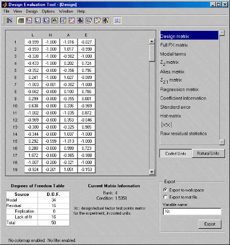
In the Design Evaluation tool you can view all the information on correlations, covariance, confounding, and variance inflation factors (VIFs). You can investigate the effects of including or excluding model terms aided by this information (you must remove them in the Stepwise window). Interpretation is aided by color-coded values based on the magnitude of the numbers. You can specify changes to these criteria.
When you open the Design Evaluation tool, the default view is a table, as shown in the preceding example. You choose the elements to display from the list on the right. Click any of the items in the list described below to change the display. Some of the items have a choice of buttons that appear underneath the list box.
To see information about each display, click the
![]() toolbar button or select View > Matrix Information.
toolbar button or select View > Matrix Information.
Table Options
You can apply color maps and filters to any items in a table view, and change the precision of the display.
To apply a color map or edit an existing one:
Select Options > Table > Colors. The Table Colors dialog box appears.
Select the check box Use a colormap for rendering matrix values.
Click the Define colormap button. The Colormap Editor dialog box appears, where you can choose how many levels to color map, and the colors and values to use to define the levels. Some tables have default color maps to aid analysis of the information, described below.
You can also use the Options > Table menu to change the precision (number of significant figures displayed) and to apply filters that remove specific values or values above or below a specific value from the display.
The status bar at bottom left displays whether color maps and filters are active in the current view.
When evaluating several designs, you can switch between them with the Next design toolbar button or the Design menu.
Design Matrix
Xn/Xc: design/actual factor test points matrix for the experiment, in natural or coded units. You can toggle between natural and coded units with the buttons on the right.
Full FX Matrix
Full model matrix, showing all possible terms in the model. You can include and exclude terms from the model here, by clicking on the green column headings. When you click one to remove a term, the column heading becomes red and the whole column is grayed.
The Full FX matrix is the same as the Jacobian for linear models if all terms included. Jacobian only includes 'in' terms. In the general case, the Jacobian is expressed:
(i, j) = df/dpj (xi)
In the case of linear models and RBFs this simplifies to:
(i,j) = jth term evaluated at ith data point = Jacobian matrix.
Model Terms
You can select terms for inclusion in or exclusion from the model here
by clicking. You can toggle the button for each term by clicking. This
changes the button from in (green) to
out (red) and vice versa. You can then view
the effect of these changes in the other displays.
Note
Removal of model terms only affects displays within the Design Evaluation tool. If you decide the proposed changes would be beneficial to your model, you must return to the Stepwise window and make the changes there to fit the new model.
Z2 Matrix
Z2: Matrix of terms that have been removed from the model. If you haven't removed any terms, the main display is blank apart from the message “All terms are currently included in the model.”
Alias Matrix
Like the Z2 matrix, the alias matrix also displays terms that are not included in the model (and is therefore not available if all terms are included in the model). The purpose of the alias matrix is to show the pattern of confounding in the design.
A zero in a box indicates that the row term (currently included in the model) is not confounded with the column term (currently not in the model). A complete row of zeros indicates that the term in the model is not confounded with any of the terms excluded from the model. A column of zeros also indicates that the column term (currently not in the model) could be included (but at the cost of a reduction in the residual degrees of freedom).
A: the alias matrix is defined by the expression
![]()
Z2.1 Matrix
As this matrix also uses the terms not included in the model, it is not available if all terms are included.
Z2.1 : Matrix defined by the expression
![]()
Regression Matrix
Regression matrix. Consists of terms included in the model.
![]() matrix where n is the number
of test points in the design and p is the number
of terms in the model.
matrix where n is the number
of test points in the design and p is the number
of terms in the model.
Coefficient Information
When you select Coefficient information, six
buttons appear below the list box. Covariance is displayed by default;
click the buttons to select any of the others for display.
Covariance. Cov(b): variance-covariance matrix for the regression coefficient vector b.
![]()
Correlation. Corr(b): correlation matrix for the regression coefficient vector b.
![]()
Correlation has a color map to aid analysis. You can view and edit the color map using Options > Table > Colors.
Partial VIFs. Variance Inflation Factors (VIFs) are a measure of the non-orthogonality of the design with respect to the selected model. A fully orthogonal design has all VIFs equal to unity.
The Partial VIFs are calculated from the off-diagonal elements of Corr(b) as
![]() for
for ![]()
Partial VIFs also has a default color map active
(<1.2 black,
>1.2<1.4
orange, >1.4 red). A filter is also
applied, removing all values within 0.1 of
1. In regular designs such as
Box-Behnken, many of the elements are exactly 1 and so need not
be displayed; this plus the color coding makes it easier for you
to see the important VIF values. You can always edit or remove
color maps and filters.
Multiple VIFs. Measure of the non-orthogonality of the design. The Multiple VIFs are defined as the diagonal elements of Corr(b):
![]()
Multiple VIFs also has a default color map active
(<8 black,
8><10 orange,
>10 red). A filter is also applied,
removing all values within 0.1 of
1. Once again this makes it easier to
see values of interest.
2 Column Corr.. Corr(X); correlation for two columns of X.
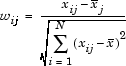
Let W denote the matrix of wij values. Then the correlation matrix for the columns of X (excluding column 1) is Corr(X), defined as
Corr(X) = W'W
2 Column Correlation has the same default color map active as Correlation.
Single Term VIFs. Measure of the nonorthogonality of the design. The Single Term VIFs are defined as
![]() for
for ![]()
Single term VIFs have a default color map active (<2 black, 2>red) and values within 0.1 of 1 are filtered out, to highlight values of interest.
Standard Error
![]() : Standard error of the
jth coefficient relative to the
RMSE.
: Standard error of the
jth coefficient relative to the
RMSE.
Hat Matrix
Full Hat matrix. H: The Hat matrix.
H = QQ'
where Q results from a QR decomposition of X. Q is an
![]() orthonormal matrix and R is an
orthonormal matrix and R is an
![]() matrix.
matrix.
Leverage values. The leverage values are the terms on the leading diagonal of H (the Hat matrix). Leverage values have a color map active (<0.8 black, 0.8>orange<0.9, >0.9 red).
|X'X|
D; determinant of X'X.
D can be calculated from the QR decomposition of X as follows:
![]()
where p is the number of terms in the currently selected model.
This can be displayed in three forms:
![]()
![]()
![]()
Raw Residual Statistic
Covariance. Cov(e): Variance-covariance matrix for the residuals.
Cov(e) = (I-H)
Correlation. Corr(e) : Correlation matrix for the residuals.
![]()
Degrees of Freedom Table
To see the Degrees of Freedom table (and the information about each
display), click the ![]() toolbar button or select View > Matrix Information.
toolbar button or select View > Matrix Information.
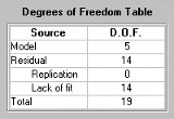
| Source | D.F. |
|---|---|
Model | p |
Residual | n-p |
Replication | by calculation |
Lack of fit | by calculation |
Total | n |
Replication is defined as follows:
Let there be nj (>1) replications at the jth replicated point. Then the degrees of freedom for replication are
![]()
and Lack of fit is given by n - p - degrees of freedom for replication.
Note: replication exists where two rows of X are identical. In regular designs the factor levels are clearly spaced and the concept of replication is unambiguous. However, in some situations spacing can be less clear, so a tolerance is imposed of 0.005 (coded units) in all factors. Points must fall within this tolerance to be considered replicated.
Design Evaluation Graphical Displays
The Design Evaluation tool has options for 1D, 2D, 3D, and 4D displays. You can switch to these by clicking the toolbar buttons or using the View menu.
Which displays are available depends on the information category selected in the list box. For the Design matrix, (with sufficient inputs) all options are available. For the Model terms, there are no display options.
You can edit the properties of all displays using the Options menu. You can configure the grid lines and background colors. In the 2D image display you can click points in the image to see their values. All 3D displays can be rotated as usual. You can edit all color map bars by double-clicking.
Export of Design Evaluation Information
All information displayed in the Design Evaluation tool can be
exported to the workspace or to a .mat file using
the radio buttons and Export button at the
bottom right. You can enter a variable name in the edit box.