View and Edit Data in the Data Editor
If you already imported data using the MBC Model Fitting app, you can open the Data Editor to view, modify, or copy the data as follows:
From the project node, in the Data Sets pane, double-click a data set.
From the project node, select Data > Edit Data, or Copy Data. If you select Copy Data, you can apply different filter or preprocessing rules to the copied data, and you can use the copied data in separate data sets.
From the test plan node, select TestPlan > Edit Data. If you edit data from a test plan, any changes to the data, such as changing filters or appending new data, are used to update the model fits and boundary models. These updates occur in parallel if you have the Parallel Computing Toolbox™.
From any modeling node, click the View Modeling Data toolbar button.
The list box at the top right contains the source file information for the
data. Other information is displayed on the left. The
Summary tab lists the numbers of records,
variables, and operating points. The bars and figures show the proportion of
records removed by any filters applied and show the number of user-defined
variables. For this example, with one user-defined variable added to a data
set originally containing seven variables, you see '7 + 1
variables.'
You can import variables, filters, and layouts from other data sets to your current project using the Tools menu. For more information, see Import Variables, Filters, and Editor Layout.
To display your data, select from one of these view types:
To change view types, use the toolbar buttons, the View menu, or right-click a view title bar.
The Operating Points Selector list pane on the left is constant for two-stage and point-by-point data, but unnecessary for one-stage data. Operating points you select apply to 2-D plots, 3-D plots, 4-D plots, pairwise plots, parallel coordinates, multiple data plots, and tables. You can right-click a 2-D plot to separate out the operating point controls. If you are viewing read-only local modeling data, the selected operating point is shown in the Operating Points pane and remains synchronized if you change operating point in the Model Browser.
By default, new data sets are called Data Object. You can
change the names of data sets at the project node by clicking a data set in
the Data Sets list or by pressing
F2.
Multiple Views
You can open multiple different views at the same time in the Data Editor. You can split views horizontally or vertically to display 2-D plots, 3-D plots, 4-D plots, pairwise plots, parallel coordinates, multiple data plots, and data tables. To split views and change view types, use the toolbar buttons, the View menu, or right-click a view title bar. Saving the data automatically saves the layout.
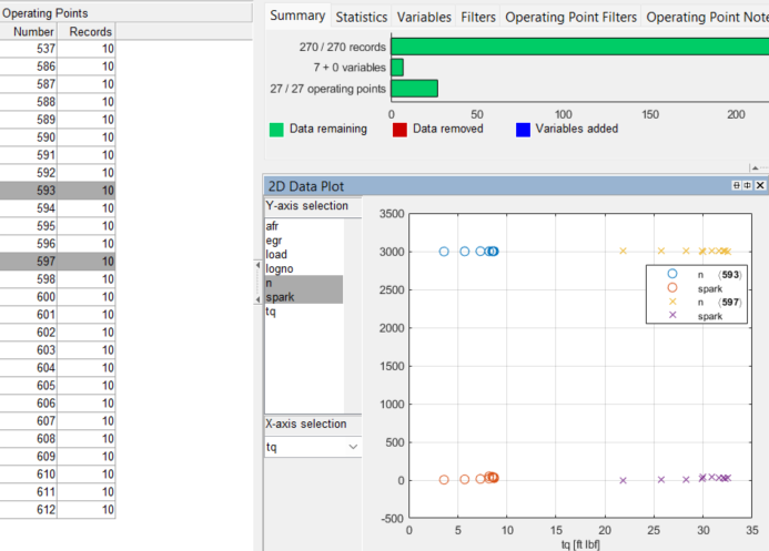
2-D Plots
In the 2-D plot view, you can select combinations of variables and operating points to plot from the list boxes on the left. You can select multiple operating points and y-axis variables to view simultaneously.
If you import one-stage data, all the data is plotted, and the Operating Points panel is not shown.

To edit data plot properties, right-click the plot and select Plot Properties. You can choose to show the legend and the grid. You can choose the line style if you want to connect the data points and the data marker point style, if any. Reorder X Data redraws the line joining the points in order from left to right. The line might not make sense when drawn in the order of the records. You can use the Show Removed Data check box to plot outliers you have removed.
Click points to select outliers, and remove them by selecting Tools > Remove Data, or use the keyboard shortcut Ctrl+A. To open a dialog box where you can choose to restore removed points, select Tools > Restore Data or use the keyboard shortcut Ctrl+Z.
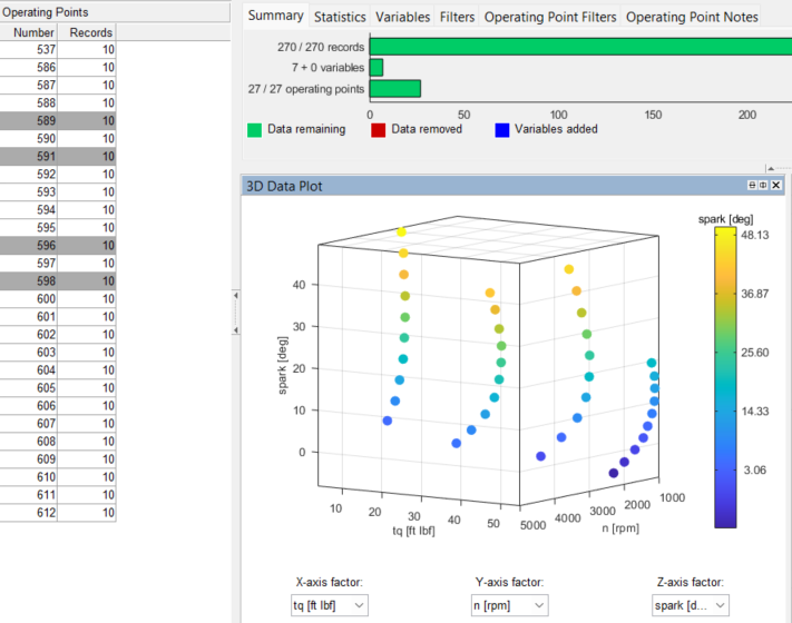
3-D Plots
In 3-D data plot views, you can select the variables for each axis from the drop-down lists, and rotate the plot by clicking and dragging. Operating points in 3-D data plots are treated similarly to operating points in 2-D plots. To edit data plot properties, you can right-click the plot and select Plot Properties. You can choose the color and style of the axes, whether to show the grid in each axis, and perspective or orthographic axes projection.
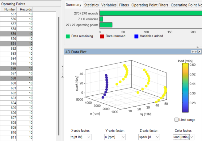
4-D Plots
In 4-D data plot views, you can select the variables for each axis from the drop-down lists, and use color as a fourth dimension by selecting a variable from the Color factor list. You can rotate the plot by clicking and dragging. To limit the data used, select the Limit range checkbox and drag over a range of values on the color bar of the fourth variable.
To edit data plot properties, you can right-click the plot and select Plot Properties. Here you can choose the color and style of the axes, whether to show the grid in each axis, and perspective or orthographic axes projection.
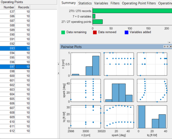
Pairwise Plots
In the pairwise plots view, you can select variables in the Select Plot Variables dialog box to create a grid of scatter plots that visualizes relationships between multiple variables. If you open the Data Editor from the test plan, the editor automatically selects inputs. If you have operating points defined, you will only get pairwise plots for the selected operating points and local inputs.
Click points on the scatter plots to select outliers. These points are highlighted in all scatter plots and 2-D plots. Remove the points by selecting Tools > Remove Data, or use the keyboard shortcut Ctrl+A. To open a dialog box where you can choose to restore removed points, select Tools > Restore Data, or use the keyboard shortcut Ctrl+Z.
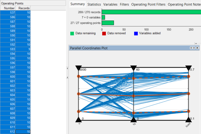
Parallel Coordinates
In the parallel coordinates view, you can select input and output variables in the Parallel Coordinate Variables dialog box to create a plot that visualizes relationships between multiple variables. If the Data Editor is opened from a test plan node, the test plan inputs are selected by default. For point-by-point test plans, the local inputs are selected.
Click on a single line to select an individual point, or click and drag the black triangle for each variable to filter out data. The filtered data points are selected on other plots, such as the pairwise plots, and can be removed from the data set. If previously filtered data is adjusted on the parallel coordinates plot, the previously filtered points are removed from the outlier selection.
For more information on parallel coordinates plots, see Explore Table Data Using Parallel Coordinates Plot.
Summary Tabs — Statistics, Variables, Filters, Operating Point Filters, and Operating Point Notes
These tabs show lists and information such as variable and filter definitions, the notes applied to filtered operating points, and the data and design points in selected clusters. Variables and Filter tabs show the definitions of each variable or filter. Double-click to select particular filters or variables to edit.
The Operating Point Notes List view shows the rules used to define
notes on the data along with the actual note, the color of the note,
and the number of operating points to which that note applies. The
specified rule is applied to each operating point in turn to decide
if that operating point should be noted. For example,
mean(TQ) > 0 evaluates the mean torque
for each operating point and notes those operating points where the
value is greater than zero.
Table View
In the Table view, you can view your data and edit and add records.
Points you have selected by clicking them in plots are outlined in red in the table. Points you have removed as outliers are light red in the table with a filter icon next to the row number. Edited cells become blue.
Tip
To view removed data in the Table view, right-click and select Allow Editing. Removed records are red.
Right-click the title bar for these options.
Duplicate Selected Records — Select one or more records, and then use this option to duplicate them. Each duplicate appears directly underneath the parent record. Edit duplicates to create new records. To use this option, you must first select Allow Editing.
Undo Edits in Selected Region — You can click and drag to highlight a region, and then use this option to reverse any edits in the highlighted area. To use this option, you must first select Allow Editing.
Allow Editing — This option toggles editing, and, as a side effect, causes all records to be shown, including those that are filtered out. Records that are filtered out appear light red in the table, with a filter icon next to the row number. You can alter records by clicking a cell and then typing a new value. Edited cells become blue. Editing the value of a cell may cause that row to be filtered out. If so, the background color of the row changes after you edit the cell.
Select Columns To Display — This option opens a dialog box where you can use the check boxes to select the columns to display in the table. Select a column, then press Ctrl+A to select all columns. Then, you can select or clear all check boxes with one click. You can click and drag column headers in the table view to rearrange columns.
Multiple Data Plots
You can add as many 2-D plots as desired to the same view, plotting the same selection of operating points in a variety of different plots. Use the right-click context menu to add and remove plots, select plot variables, and edit plot properties. You can select single or multiple Y variables to plot against a single X variable (or no X variable) in the Plot Variables dialog box. Select operating points to display in the list on the left of the Data Editor, as for 2-D and 3-D plots and the Table view.
Note that you can select different plot properties and variables for each plot within the Multiple Data Plots view. Click or right-click to select a plot before selecting Plot Variables or Plot Properties. For each plot, you can use the same plot properties options as for the single 2-D data plots. You can choose to show the legend and the grid. You can choose the line style if you want to connect the data points and the data marker point style, if any. Reorder X Data redraws the line joining the points in order from left to right. The line might not make sense when drawn in the order of the records. To view removed data in the Multiple Data Plots, select Plot Properties and select Show removed data.
Click points to select outliers, and remove them by selecting Tools > Remove Data, or use the keyboard shortcut Ctrl+A. Selected outliers are outlined in red.
To open a dialog box where you can choose to restore removed points, select Tools > Restore Data, or use the keyboard shortcut Ctrl+Z.
Design Match Plots
You use these views for matching data to design points. Use the list in the Design Match view to examine your data and design. Click points in the plot to select them across the Data Editor. The selected points are displayed in the table view and other data plot views (except 2-D plots, which have separate controls).