Estimate GNSS Receiver Position with Simulated Satellite Constellations

This example uses:

Track the position of a ground vehicle using a simulated Global Navigation Satellite System (GNSS) receiver. The satellites are simulated using the satelliteScenario (Satellite Communications Toolbox) object, the satellite signal processing of the receiver are simulated using the lookangles and pseudoranges functions, and the receiver position is estimated with the receiverposition function.

Overview

This example focuses on the space segment, or satellite constellations, and the GNSS sensor equipment for a satellite system. To obtain an estimate of the GNSS receiver position, the navigation processor requires the satellite positions from the space segment and the pseudoranges from the ranging processor in the receiver.

Specify Simulation Parameters

Load the MAT-file that contains the ground-truth position and velocity of a ground vehicle travelling toward the Natick, MA campus of The MathWorks, Inc.

Specify the start, stop, and sample time of the simulation. Also, specify the mask angle, or minimum elevation angle, of the GNSS receiver. Finally, specify the RINEX navigation message file for the initial satellite orbital parameters.

% Load ground truth trajectory.
load("routeNatickMA.mat","lat","lon","pos","vel","lla0");
recPos = pos;
recVel = vel;

% Specify simulation times.
startTime = datetime(2021,6,24,8,0,0,"TimeZone","America/New_York");
simulationSteps = size(pos,1);
dt = 1;
stopTime = startTime + seconds((simulationSteps-1)*dt);

% Specify mask angle.
maskAngle = 5; % degrees

% Convert receiver position from north-east-down (NED) to geodetic
% coordinates.
receiverLLA = ned2lla(recPos,lla0,"ellipsoid");

% Specify the RINEX file.
rinexFile = "GODS00USA_R_20211750000_01D_GN.rnx";

% Set RNG seed to allow for repeatable results. 
rng("default");

Visualize the geoplot for the ground truth trajectory.

figure
geoplot(lat,lon)
geobasemap("topographic")
title("Ground Truth Trajectory")

Figure contains an axes object with type geoaxes. The geoaxes object contains an object of type line.

Simulate Satellite Positions Over Time

The satelliteScenario object enables you to specify initial orbital parameters and visualize them using the satelliteScenarioViewer object. This example uses the satelliteScenario and a RINEX file with initial orbital parameters to simulate the GPS constellations over time. Alternatively, you could use the gnssconstellation object which simulates satellite positions using nominal orbital parameters or a RINEX file, and only the current simulation time is needed to calculate the satellite positions.

% Create scenario.
sc = satelliteScenario(startTime, stopTime, dt);

% Initialize satellites. 
navmsg = rinexread(rinexFile);
satellite(sc,navmsg);
satID = sc.Satellites.Name;

% Preallocate results.
numSats = numel(sc.Satellites);
allSatPos = zeros(numSats,3,simulationSteps);
allSatVel = zeros(numSats,3,simulationSteps);

% Save satellite states over entire simulation.
for i = 1:numel(sc.Satellites)
    [oneSatPos, oneSatVel] = states(sc.Satellites(i),"CoordinateFrame","ecef");
    allSatPos(i,:,:) = permute(oneSatPos,[3 1 2]);
    allSatVel(i,:,:) = permute(oneSatVel,[3 1 2]);
end

Calculate Pseudoranges

Use the satellite positions to calculate the pseudoranges and satellite visibilities throughout the simulation. The mask angle is used to determine the satellites that are visible to the receiver. The pseudoranges are the distances between the satellites and the GNSS receiver. The term pseudorange is used because this distance value is calculated by multiplying the time difference between the current receiver clock time and the timestamped satellite signal by the speed of light.

% Preallocate results.
allP = zeros(numSats,simulationSteps);
allPDot = zeros(numSats,simulationSteps);
allIsSatVisible = false(numSats,simulationSteps);

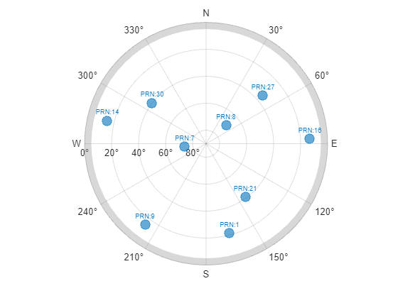
% Use the skyplot to visualize satellites in view.
sp = skyplot([],[],MaskElevation=maskAngle);

for idx = 1:simulationSteps
    satPos = allSatPos(:,:,idx);
    satVel = allSatVel(:,:,idx);
    
    % Calculate satellite visibilities from receiver position.
    [satAz,satEl,allIsSatVisible(:,idx)] = lookangles(receiverLLA(idx,:),satPos,maskAngle);
    
    % Calculate pseudoranges and pseudorange rates using satellite and
    % receiver positions and velocities.
    [allP(:,idx),allPDot(:,idx)] = pseudoranges(receiverLLA(idx,:),satPos,recVel(idx,:),satVel);
    
    set(sp,"AzimuthData",satAz(allIsSatVisible(:,idx)), ...
        "ElevationData",satEl(allIsSatVisible(:,idx)), ...
        "LabelData",satID(allIsSatVisible(:,idx)))
    drawnow limitrate
end

Figure contains an object of type skyplot.

Estimate Receiver Position from Pseudoranges and Satellite Positions

Finally, use the satellite positions and pseudoranges to estimate the receiver position with the receiverposition function.

% Preallocate results.
lla = zeros(simulationSteps,3);
gnssVel = zeros(simulationSteps,3);
hdop = zeros(simulationSteps,1);
vdop = zeros(simulationSteps,1);

for idx = 1:simulationSteps
    p = allP(:,idx);
    pdot = allPDot(:,idx);
    isSatVisible = allIsSatVisible(:,idx);
    satPos = allSatPos(:,:,idx);
    satVel = allSatVel(:,:,idx);
    
    % Estimate receiver position and velocity using pseudoranges,
    % pseudorange rates, and satellite positions and velocities.
    [lla(idx,:),gnssVel(idx,:),hdop(idx,:),vdop(idx,:)] = receiverposition(p(isSatVisible),...
        satPos(isSatVisible,:),pdot(isSatVisible),satVel(isSatVisible,:));
end

Visualize Results

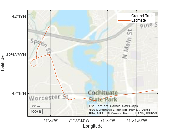
Plot the ground truth position and the estimated receiver position on a geoplot.

figure
geoplot(lat,lon,lla(:,1),lla(:,2))
geobasemap("topographic")
legend("Ground Truth","Estimate")

Figure contains an axes object with type geoaxes. The geoaxes object contains 2 objects of type line. These objects represent Ground Truth, Estimate.

Plot the absolute error in the position estimate. The error is smoothed by a moving median to make the plot more readable. The error in the x- and y-axis is smaller because there are satellites on either side of the receiver. The error in the z-axis is larger because there are only satellites above the receiver, not below it. The error changes over time as the receiver moves and some satellites come in and out of view.

estPos = lla2ned(lla,lla0,"ellipsoid");
winSize = floor(size(estPos,1)/10);
figure
plot(smoothdata(abs(estPos-pos),"movmedian",winSize))
legend("x","y","z")
xlabel("Time (s)")
ylabel("Error (m)")
title("Position (NED) Error")

Figure contains an axes object. The axes object with title Position (NED) Error, xlabel Time (s), ylabel Error (m) contains 3 objects of type line. These objects represent x, y, z.