Fuse Multiple Lidar Sensors Using Map Layers
Occupancy maps offer a simple yet robust way of representing an environment for robotic applications by mapping the continuous world-space to a discrete data structure. Individual grid cells can contain binary or probabilistic information about obstacle information. However, an autonomous platform may use a variety of sensors that may need to be combined to estimate both the current state of the platform and the state of the surrounding environment.
This example focuses on integrating a variety of sensors to estimate the state of the environment and store occupancy values are different map layers. The example shows how the multiLayerMap object can be used to visualize, debug, and fuse data gathered from three lidar sensors mounted to an autonomous vehicle. The sensor readings in this example are simulated using a set of lidarPointCloudGenerator (Automated Driving Toolbox) objects which capture readings from the accompanying drivingScenario (Automated Driving Toolbox) object.
Each lidar updates its own validatorOccupancyMap3D object which enables us to visualize the local map created by each sensor in isolation. These local maps can be used to quickly identify sources of noise or mounting error, and can help in choosing an appropriate fusion technique. The multiLayerMap contains a fourth mapLayer object, which uses a custom callback function to fuse the data contained in each occupancy layer. Lastly, the fused map is used to update the corresponding subregion of a world map as the autonomous vehicle moves along the preplanned path.
Load Driving Scenario
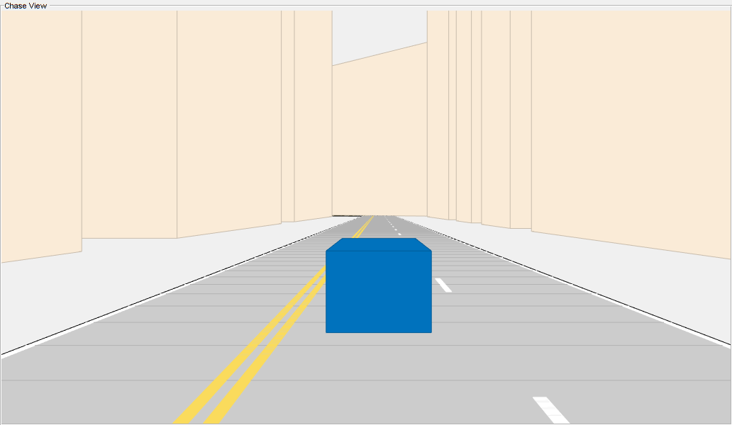
First, create a drivingScenario object and populate the scene with several buildings using an example helper function. The function also visualizes the scene.
scene = drivingScenario;
groundTruthVehicle = vehicle(scene,'PlotColor',[0 0.4470 0.7410]);

% Add a road and buildings to scene and visualize.
exampleHelperPopulateScene(scene,groundTruthVehicle);
Generate a trajectory that follows the main road in the scene using a waypointTrajectory object.
sampleRate = 100;
speed = 10;
t = [0 20 25 44 46 50 54 56 59 63 90].';
wayPoints = [  0   0 0;
             200   0 0;
             200  50 0;
             200 230 0;
             215 245 0;
             260 245 0;
             290 240 0;
             310 258 0;
             290 275 0;
             260 260 0;
             -15 260 0];
velocities = [ speed     0 0;
               speed     0 0;
                   0 speed 0;
                   0 speed 0;
               speed     0 0;
               speed     0 0;
               speed     0 0;
                   0 speed 0;
              -speed     0 0;
              -speed     0 0;
              -speed     0 0];

traj = waypointTrajectory(wayPoints,'TimeOfArrival',t,...
    'Velocities',velocities,'SampleRate',sampleRate);
Create Simulated Lidar Sensors
To gather lidar readings from the driving scenario, create three lidarPointcloudGenerator objects using an example helper function. This vehicle has been configured to have two front-facing, narrow field-of-view (FOV) lidars and a single wide FOV rear-facing Lidar. The overlapping region of both front-facing sensors should help to quickly register and confirm free space ahead of the vehicle, whereas the rear-facing sensor range helps map the traversed region.
lidarSensors = exampleHelperCreateVehicleSensors(scene, groundTruthVehicle);
disp(lidarSensors)
{1×1 lidarPointCloudGenerator} {1×1 lidarPointCloudGenerator} {1×1 lidarPointCloudGenerator}
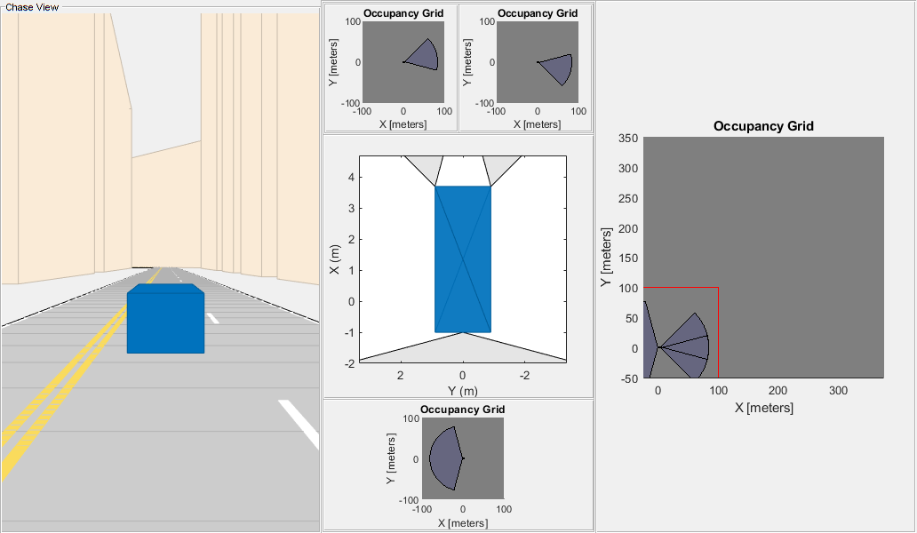
Initialize Egocentric Map
Create a multiLayerMap object composed of three occupancyMap objects and one generic mapLayer object. Each local occupancyMap is updated by the corresponding lidar sensor. To combine data from all maps into the mapLayer object, set the GetTransformFcn name-value argument to the exampleHelperFuseOnGet function stored as a handle fGet. The exampleHelperFuseOnGet function fused all three maps data values by calling the getMapData function on each and using a log-odds summation of the values.
% Define map and parameters.
res = 2;
width = 100*2;
height = 100*2;

% Define equal weights for all sensor readings.
weights = [1 1 1];

% Create mapLayers for each sensor.
fLeftLayer  = occupancyMap(width,height,res,'LayerName','FrontLeft');
fRightLayer = occupancyMap(width,height,res,'LayerName','FrontRight');
rearLayer   = occupancyMap(width,height,res,'LayerName','Rear');

% Create a get callback used to fuse data in the three layers.
fGet = @(obj,values,varargin)...
    exampleHelperFuseOnGet(fLeftLayer,fRightLayer,rearLayer,...
                        weights,obj,values,varargin{:});

% Create a generic mapLayer object whose getMapData function fuses data from all
% three layers.
fusedLayer = mapLayer(width,height,'Resolution',res,'LayerName','FuseLayer',...
                    'GetTransformFcn',fGet,'DefaultValue',0.5);

% Combine layers into a multiLayerMap.
egoMap = multiLayerMap({fLeftLayer, fRightLayer, rearLayer, fusedLayer});

% Set map grid origin so that the robot is located at the center.
egoMap.GridOriginInLocal = -[diff(egoMap.XLocalLimits) diff(egoMap.YLocalLimits)]/2;
Create Reconstruction Map
Create an empty world map. This map is periodically updated using data from the fusion layer. Use this map to indicate how well the lidar fusion method is working.
% Create an empty reconstruction layer covering the same area as world map.
reconLayer = occupancyMap(400,400,res,... % width,height,resolution
    'LayerName','FuseLayer','LocalOriginInWorld',[-25 -50]);
Setup Visualization
Plot the egocentric layers next to the reconstructed map. Use the exampleHelperShowEgoMap function to display each local map.
% Setup the display window.
axList = exampleHelperSetupDisplay(groundTruthVehicle,lidarSensors);

% Display the reconstructionLayer and submap region.
show(reconLayer,'Parent', axList{1});
hG = findobj(axList{1},'Type','hggroup');
egoOrientation = hG.Children;
egoCenter = hgtransform('Parent',hG);
egoOrientation.Parent = egoCenter;
gridLoc = egoMap.GridLocationInWorld;
xLimits = egoMap.XLocalLimits;
yLimits = egoMap.YLocalLimits;
rectangle('Parent',egoCenter,...
    'Position',[gridLoc diff(xLimits) diff(yLimits)],...
    'EdgeColor','r');

% Display the local maps built by each sensor alongside the reconstruction map.
exampleHelperShowEgoMap(axList,egoMap,[0 0 0],{'FrontLeft Lidar','FrontRight Lidar','Rear Lidar','Fused'});

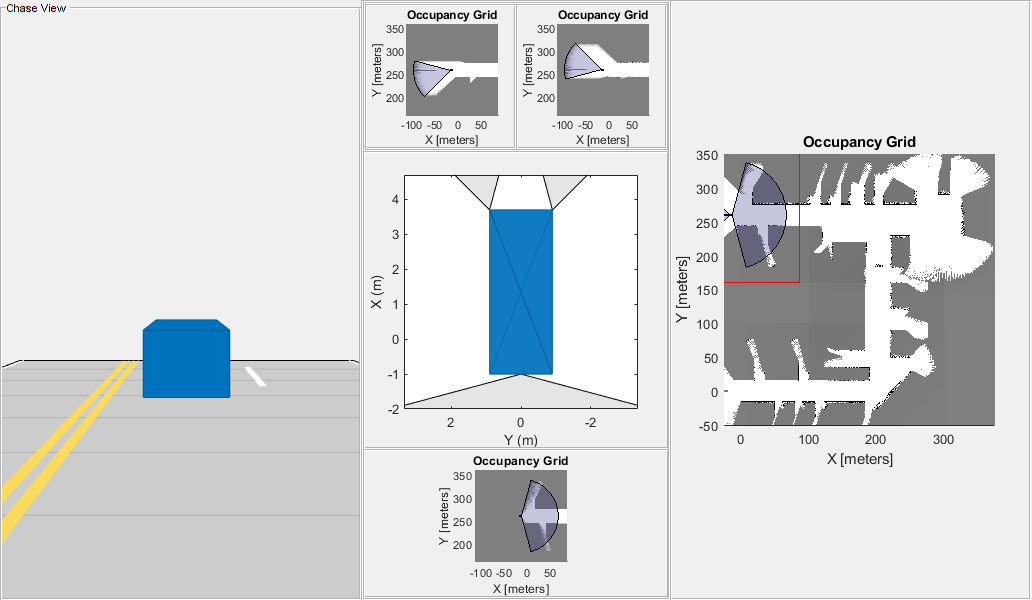
Simulate Sensor Readings and Build Map
Move the robot along the trajectory while updating the map with the simulated Lidar readings.
To run the driving scenario, call the exampleHelperResetSimulation helper function. This resets the simulation and trajectory, clears the map, and moves the egocentric maps back to the first point of the trajectory.
exampleHelperResetSimulation(scene,traj,lidarSensors,egoMap,reconLayer)
Call the exampleHelperRunSimulation function to execute the simulation.
The primary operations of the simulation loop are:
Get the next pose in the trajectory from
trajand extract the z-axis orientation (theta) from the quaternion.Move the
egoMapto the new[x y theta]pose.Retrieve sensor data from the
lidarPointCloudGenerators.Update the local maps with sensor data using
insertRay.Update the global map using the
mapLayerfused result.Refresh the visualization.
exampleHelperRunSimulation(scene,traj,groundTruthVehicle,egoMap,lidarSensors,reconLayer,axList)

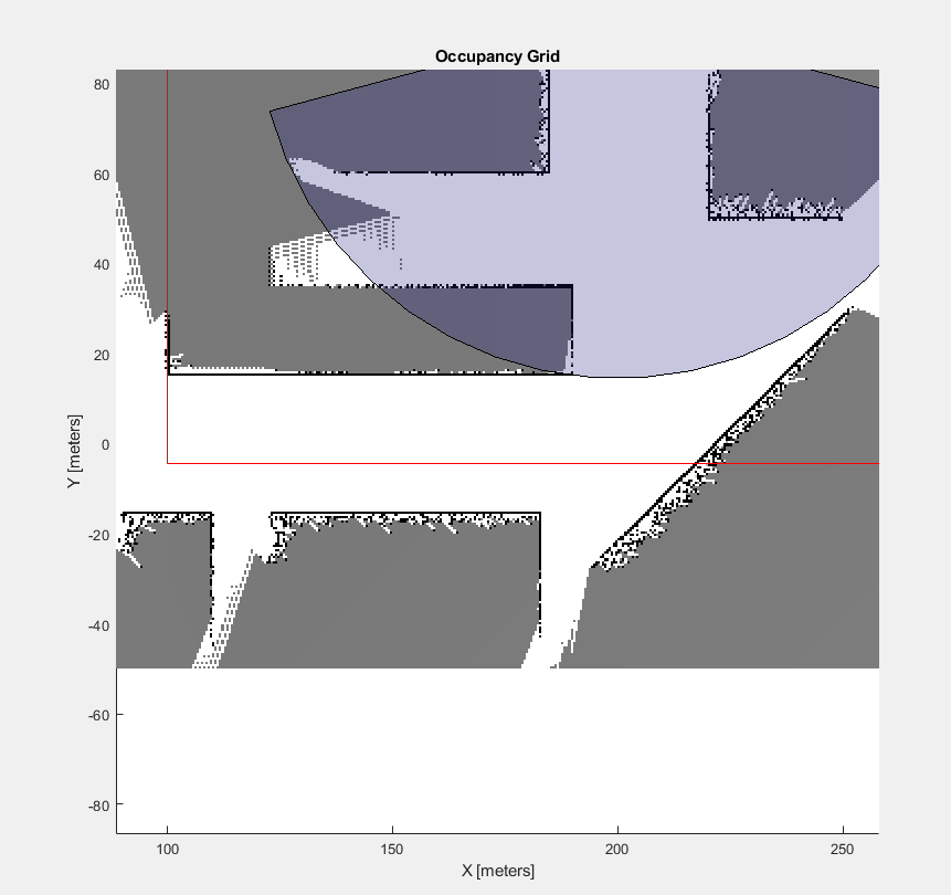
The displayed results indicate that the front-right sensor is introducing large amounts of noise into the fused map. Notice that the right-hand wall has more variability throughout the trajectory. You do not want to discard readings from this sensor entirely because the sensor is still detecting free space in the front. Instead reduce the weight of those sensor readings during fusion and recreate the full multilayer map. Then, reset and rerun the simulation.
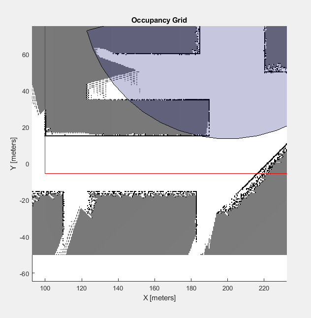
% Construct a new multiLayerMap with a different set of fusion weights
updatedWeights = [1 0.25 1];
egoMap = exampleHelperConstructMultiLayerEgoMap(res,width,height,updatedWeights);

% Rerun the simulation
exampleHelperResetSimulation(scene,traj,lidarSensors,egoMap,reconLayer)
exampleHelperRunSimulation(scene,traj,groundTruthVehicle,egoMap,lidarSensors,reconLayer,axList)
After simulating again, notice a few things about the map:
Regions covered only by the noisy sensor can still detect freespace with little noise.
While noise is still present, the readings from the other sensors outweigh those from the noisy sensor. The map shows distinct obstacle boundaries (black squares) in regions of sensor overlap.
Noise beyond the distinct boundaries remain because the noisy lidar is the only sensor that reports readings in those areas, but does not connect to other free space.
Next Steps
This example shows a simple method of how readings can be fused. You may further customize this fusion with the following suggestions:
To adjust weights based on sensor confidence prior to layer-layer fusion, specify a custom inverse sensor model when using the
insertRayobject function in theexamplerHelperUpdateEgoMapfunction.To assign occupancy values based on a more complex confidence distribution like a gaussian inverse model, use the
raycastobject function to retrieve the cells traced by each emanating ray. Once a set of cells has been retrieved, values can be explicitly assigned based on more complex methods.To reduce confidence of aging cells, utilize additional map layers which keep track of timestamps for each cell. These timestamps can be used to place greater importance on recently updates cells and slowly ignore older readings.