Ground Vehicle Pose Estimation for Tightly Coupled IMU and GNSS
This example shows how to estimate the position and orientation of a ground vehicle by building a tightly coupled extended Kalman filter and using it to fuse sensor measurements. A tightly coupled filter fuses inertial measurement unit (IMU) readings with raw global navigation satellite system (GNSS) readings. In contrast, a loosely coupled filter fuses IMU readings with filtered GNSS receiver readings.
Loosely Coupled Filter Diagram
Tightly Coupled Filter Diagram
Though a tightly coupled filter requires additional processing, you can use it when fewer than four GNSS satellite signals are available, or when some satellite signals are corrupted by interference such as multipath noise. This type of noise can occur when a ground vehicle is traveling through a portion of road with many obstructions, such as an urban canyon, where many surfaces reflect a combination of signals back into the receiver and interfere with the direct signal. Because the ground vehicle is in an urban environment with a lot of opportunity for multipath noise, this example uses a tightly coupled filter.
Define Filter Input
Specify these parameters for the sensor simulation:
Trajectory motion quantities
IMU sampling rate
GNSS receiver sampling rate
RINEX navigation message file
The RINEX navigation message file contains GNSS satellite orbital parameters used to compute satellite positions and velocities. The satellite positions and velocities are important for generating the GNSS pseudoranges and pseudorange rates.
load("routeNatickMATightlyCoupled","pos","orient","vel","acc","angvel","lla0","imuFs","gnssFs");
navfilename = "GODS00USA_R_20211750000_01D_GN.rnx";
Create the IMU sensor object. Set the axes misalignment and constant bias values to 0 to simulate calibration.
imu = imuSensor(SampleRate=imuFs);
loadparams(imu,"generic.json","GenericLowCost9Axis");
imu.Accelerometer.AxesMisalignment = 100*eye(3);
imu.Accelerometer.ConstantBias = [0 0 0];
imu.Gyroscope.AxesMisalignment = 100*eye(3);
imu.Gyroscope.ConstantBias = [0 0 0];
Read the RINEX file by using the rinexread function. Use only the first set of GPS satellites from the file, and set the initial time for the simulation to the first time step in the file.
data = rinexread(navfilename);
[~,idx] = unique(data.GPS.SatelliteID);
navmsg = data.GPS(idx,:);
t0 = navmsg.Time(1);
Load the noise parameters, paramsTuned, for the IMU sensor and GNSS receiver from the tunedNoiseParameters MAT file.
load("tunedNoiseParameters.mat","paramsTuned");
accelNoise = paramsTuned.AccelerometerNoise;
gyroNoise = paramsTuned.GyroscopeNoise;
pseudorangeNoise = paramsTuned.exampleHelperINSGNSSNoise(1);
pseudorangeRateNoise = paramsTuned.exampleHelperINSGNSSNoise(2);
Set the RNG seed to produce repeatable results.
rng defaultCreate Filter and Filter Sensor Models
To create the tightly coupled filter by using the insEKF object, you must define the conversion of filter states to raw GNSS measurements. Use the exampleHelperINSGNSS helper function to define this conversion.
gnss = exampleHelperINSGNSS;
gnss.ReferenceLocation = lla0;
Define an IMU model by creating accelerometer and gyroscope models using the insAccelerometer and insGyroscope objects, respectively.
accel = insAccelerometer;
gyro = insGyroscope;
Create the filter by using the IMU sensor model, the raw GNSS sensor model, and a 3-D pose motion model represented as an insMotionPose object.
filt = insEKF(accel,gyro,gnss,insMotionPose);
Set the initial states of the filter using tuned parameters from paramsTuned.
filt.State = paramsTuned.InitialState;
filt.StateCovariance = paramsTuned.InitialStateCovariance;
filt.AdditiveProcessNoise = paramsTuned.AdditiveProcessNoise;
Estimate Vehicle Pose
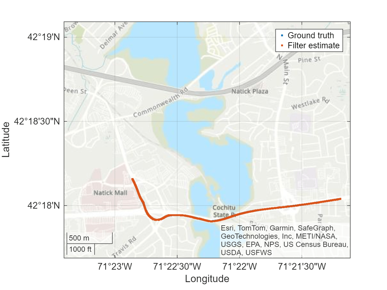
Create a figure in which to view the position estimate for the ground vehicle during the filtering process.
figure
posLLA = ned2lla(pos,lla0,"ellipsoid");
geoLine = geoplot(posLLA(1,1),posLLA(1,2),".",posLLA(1,1),posLLA(1,2),".");
geolimits([42.2948 42.3182],[-71.3901 -71.3519])
geobasemap topographic
legend("Ground truth","Filter estimate")
Allocate a matrix in which to store the position estimate results.
numSamples = size(pos,1);
estPos = NaN(numSamples,3);
estOrient = ones(numSamples,1,"quaternion");
imuSamplesPerGNSS = imuFs/gnssFs;
numGNSSSamples = numSamples/imuSamplesPerGNSS;
Set the current simulation time to the specified initial time.
t = t0;
Fuse the IMU and raw GNSS measurements. In each iteration, fuse the accelerometer and gyroscope measurements to the GNSS measurements separately to update the filter states, with the covariance matrices defined by the previously loaded noise parameters. After updating the filter state, log the new position and orientation states. Finally, predict the filter states to the next time step.
for ii = 1:numGNSSSamples
    for jj = 1:imuSamplesPerGNSS
        imuIdx = (ii-1)*imuSamplesPerGNSS + jj;
        [accelMeas,gyroMeas] = imu(acc(imuIdx,:),angvel(imuIdx,:),orient(imuIdx,:));

        fuse(filt,accel,accelMeas,accelNoise);
        fuse(filt,gyro,gyroMeas,gyroNoise);

        estPos(imuIdx,:) = stateparts(filt,"Position");
        estOrient(imuIdx,:) = quaternion(stateparts(filt,"Orientation"));

        t = t + seconds(1/imuFs);
        predict(filt,1/imuFs);
    end
Update the satellite positions and raw GNSS measurements.
    gnssIdx = ii*imuSamplesPerGNSS;
    recPos = posLLA(gnssIdx,:);
    recVel = vel(gnssIdx,:);
    [satPos,satVel,satIDs] = gnssconstellation(t,"RINEXData",navmsg);
    [az,el,vis] = lookangles(recPos,satPos);
    [p,pdot] = pseudoranges(recPos,satPos(vis,:),recVel,satVel(vis,:));
    z = [p; pdot];
Update the satellite positions on the GNSS model.
    gnss.SatellitePosition = satPos(vis,:);
    gnss.SatelliteVelocity = satVel(vis,:);
Fuse the raw GNSS measurements.
    fuse(filt,gnss,z, ...
        [pseudorangeNoise*ones(1,numel(p)),pseudorangeRateNoise*ones(1,numel(pdot))]);
    estPos(gnssIdx,:) = stateparts(filt,"Position");
    estOrient(gnssIdx,:) = quaternion(stateparts(filt,"Orientation"));
Update the position estimation plot.
    estPosLLA = ned2lla(estPos,lla0,"ellipsoid");
    set(geoLine(1),LatitudeData=posLLA(1:gnssIdx,1),LongitudeData=posLLA(1:gnssIdx,2));
    set(geoLine(2),LatitudeData=estPosLLA(1:gnssIdx,1),LongitudeData=estPosLLA(1:gnssIdx,2));
    drawnow limitrate
end

Validate Results
Calculate the RMS error to validate the results. The tightly coupled filter uses the provided sensor readings to estimate the ground vehicle pose with a relatively low RMS error.
posDiff = estPos - pos;
posRMS = sqrt(mean(posDiff.^2));
disp(['3-D Position RMS Error — X: ',num2str(posRMS(1)),', Y:', ...
    num2str(posRMS(2)),', Z: ',num2str(posRMS(3)),' (m)'])
3-D Position RMS Error - X: 0.8522, Y:0.62864, Z: 0.9633 (m)
orientDiff = rad2deg(dist(estOrient,orient));
orientRMS = sqrt(mean(orientDiff.^2));
disp(['Orientation RMS Error — ',num2str(orientRMS),' (degrees)'])
Orientation RMS Error - 4.0385 (degrees)