优化绿色氢气生产系统

此示例使用:

打开实时脚本

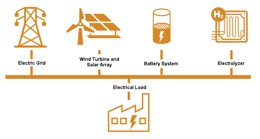
此示例展示了如何确定电解器生产氢气的绿色系统的关键组件尺寸。关键组件如下：

太阳能电池板
风力发电机
电池系统
双向连接电网
生产氢气 (H2) 的电解器
电气负载

该图说明了各个组件的电气连接方式。

使用技术经济分析来确定最佳组件尺寸。技术考虑包括绿色氢气生产系统的物理和操作约束。使用净现值 (NPV)评估投资该系统的经济可行性。假设折现率为 5%。后面的示例中，您可以检查不同折现率的效果。

问题数据

加载以下 20 年期间每小时数据的数据集：

负载功率 (kW)
电网电价（美元/千瓦）
太阳能概况（标准化为 [0 1]）
风能概况（标准化为 [0 1]）
绿氢价格（美元/公斤）

实际上，这种类型的数据可能来自公共或内部数据源，或来自预测或预报模型。对于此示例，将代表性合成数据加载到单个数据结构中（为了方便）。

loadPower = load("loadPower.mat");
priceGrid = load("priceGrid.mat");
priceH2 = load("priceH2.mat");
solarProfile = load("solarProfile.mat");
windProfile = load("windProfile.mat");

data = struct(loadPower=loadPower.loadPower,...
    priceGrid=priceGrid.priceGrid,...
    priceH2=priceH2.priceH2,...
    solarProfile=solarProfile.solarProfile,...
    windProfile=windProfile.windProfile);

clear loadPower priceGrid priceH2 solarProfile windProfile

numYears = 20;
numSteps = 24*365*numYears; % Ignore the effects of leap years and seconds.
timeStep = 1; % unit = hours. Convert from power to energy by multiplying by timeStep.

对于 NPV 计算，假设年折现率为 5%。

discount_rate = 0.05;

电力消耗和生产建模

对系统的每个组件进行建模。首先创建一个最大化优化问题，其中目标是 NPV（在示例后面指定）。

H2productionProblem = optimproblem(ObjectiveSense="maximize");

将所有变量视为连续变量。

电网电力

创建一个名为 gridPower 的优化变量向量，表示电网电力的使用情况。

假设该系统可以使用来自电网的高达 100 kW 的电力，并且该系统还可以向电网回馈高达 10 kW 的电力。因此，该系统既可以从电网购买电力，也可以将电力卖回给电网。
假设从电网购买电力和将电力卖回给电网的价格相同。

gridPowerBuyLimit = 100; % kW
gridPowerSellLimit = -10; % kW - negative value to indicate selling back to grid
gridPower = optimvar("gridPower",numSteps,...
    LowerBound=gridPowerSellLimit,UpperBound=gridPowerBuyLimit);

太阳能

创建一个名为 solarRating 的优化变量向量，表示太阳能发电的容量。

假设单个太阳能装置的最大功率为 solarRating，其中 solarRating 是一个不超过 500 kW 的优化变量。
太阳能每小时的产量是 data.solarProfile*solarRating。
太阳能装置的成本与其额定功率成正比。

solarPowerCost = 1500; % $/kW of capacity, so total cost = solarPowerCost*solarRating.

太阳能装置的成本取自 https://atb.nrel.gov/electricity/2021/residential_pv。

maxSolarRating = 500; % kW
solarRating = optimvar("solarRating",LowerBound=0,UpperBound=maxSolarRating);

风力

创建一个名为 windRating 的优化变量向量，表示风力发电的容量。

假设单个风力发电机组的最大功率为 windRating，其中 windRating 是一个不超过 500 kW 的优化变量。
风力发电的每小时产量是 data.windProfile*windRating。
风力发电机组的成本与其额定功率成正比。

windPowerCost = 1500; % $/kW of capacity, so total cost = windPowerCost*windRating.
maxWindRating = 500; % kW
windRating = optimvar("windRating",LowerBound=0,UpperBound=maxWindRating);

电力储存

对电力容量（单位时间内存储或存储外的能量）和总能量容量进行建模。

假设电源容量为 storagePowerRating，这是一个不超过 200 kW 的优化变量。
假设单个存储单元的最大能量容量为 storageEnergyRating，优化变量不超过 10,000 kWh。

存储单元的成本包括三个部分：

固定成本为 5982 美元
每千瓦发电容量成本为 1690 美元
每千瓦时能源成本为 354 美元

这些成本取自 https://atb.nrel.gov/electricity/2021/residential_battery_storage。

storageFixedCost = 5982;   % $ one-time cost
storagePowerCost = 1690;   % $/kW
storageEnergyCost = 354;   % $/kWh

为存储单元创建优化变量。创建 storagePower 作为表示每个时间步的功率的向量，以及创建 storageEnergy 作为表示每个时间步的能量的向量。另外，创建标量变量 storagePowerRating 和 storageEnergyRating 分别表示电力和能量的容量。

maxStoragePowerRating = 200; % kW
maxStorageEnergyRating = 10e3; % kWh
storagePower  = optimvar("storagePower",numSteps,...
    LowerBound=-maxStoragePowerRating,UpperBound=maxStoragePowerRating);
storageEnergy = optimvar("storageEnergy",numSteps,...
    LowerBound=0,UpperBound=maxStorageEnergyRating);
storagePowerRating = optimvar("storagePowerRating",LowerBound=0,UpperBound=maxStoragePowerRating);
storageEnergyRating = optimvar("storageEnergyRating",LowerBound=0,UpperBound=maxStorageEnergyRating);

功率和能量变量通过能量平衡相关：一小时内使用或获得的功率导致储存的能量减少或增加。通过创建优化约束来强制实现这种能量平衡。

storageEnergyBalance = optimconstr(numSteps); % Initialize
storageEnergyBalance(1) = storageEnergy(1) == -storagePower(1)*timeStep; % Initialize assuming zero stored energy at first
storageEnergyBalance(2:numSteps)   =  storageEnergy(2:numSteps) == ...
    storageEnergy(1:numSteps-1) - storagePower(2:numSteps)*timeStep;
H2productionProblem.Constraints.storageEnergyBalance = storageEnergyBalance;

存储系统会随着时间的推移慢慢退化。对存储系统的退化进行建模，在系统的整个生命周期内，存储容量和功率限制都会呈 5% 的线性下降。

degradationFactor = linspace(1,1-0.05,numSteps)';
H2productionProblem.Constraints.chargeUpper = ...
    storageEnergy <= storageEnergyRating*degradationFactor;
H2productionProblem.Constraints.storagePowerLower1 = ...
    storagePower  >= -storagePowerRating*degradationFactor;
H2productionProblem.Constraints.storagePowerUpper = ...
    storagePower  <= storagePowerRating*degradationFactor;

限制存储能量仅使用风能或太阳能，而不是来自电网的能量。这一约束确保了存储单元在生产氢气期间仅提供来自可再生能源的能源。

renewablePower = data.solarProfile*solarRating + data.windProfile*windRating;
H2productionProblem.Constraints.storagePowerLower2 = storagePower >= -renewablePower;

电解器装置

创建一个名为 electrolyzerPower 的优化变量，表示电解器每小时使用的电量，并创建一个名为 electrolyzerPowerRating 的优化变量，表示 electrolyzerPower 的最大值。

假设有一个电解器装置。
电解器的额定功率可在 0 至 50kW 之间。
电解器连续生产氢气，并每周出售储存的氢气。
系统中储存氢气的成本尚未考虑。
电解器使用 55 千瓦时的电能来生产 1 公斤氢气。
电解器装置的成本与其功率容量成正比。

electrolyzerPowerCost = 4000; % $/kW of capacity, so total cost = electrolyzerPowerCost*electrolyzerPowerRating.

为电解器参数创建变量。

maxElectrolyzerPowerRating = 50; % kW
H2SellInterval = 24*7; % hours in one week
H2ProdEnergy = 55; % kWh/kg

为每个时间步长的电解器功率和储存的氢气创建优化变量。

electrolyzerPower  = optimvar("electrolyzerPower",numSteps,...
    LowerBound=0,UpperBound=maxElectrolyzerPowerRating);
electrolyzerPowerRating = optimvar("electrolyzerPowerRating",LowerBound=0,UpperBound=maxElectrolyzerPowerRating);
H2_stored = optimvar("H2_stored",numSteps,LowerBound=0,UpperBound=1e12);

制定约束，强制使用电解器电力来生产氢气。

electrolyzerH2prod = optimconstr(numSteps);
electrolyzerH2prod(1) = H2_stored(1) == electrolyzerPower(1)*timeStep/H2ProdEnergy;
electrolyzerH2prod(2:numSteps) = H2_stored(2:numSteps) == ...
    H2_stored(1:numSteps-1) + electrolyzerPower(2:numSteps)*timeStep/H2ProdEnergy;
H2productionProblem.Constraints.electrolyzerH2prod = electrolyzerH2prod;

创建一个约束，即所有生产的氢气都按照指定的时间间隔出售。

H2productionProblem.Constraints.electrolyzerH2prod(H2SellInterval+1:H2SellInterval:numSteps) = ...
    H2_stored(H2SellInterval+1:H2SellInterval:numSteps) == ...
    electrolyzerPower(H2SellInterval+1:H2SellInterval:numSteps)*timeStep/H2ProdEnergy;

计算在指定的销售间隔内销售了多少氢气。

H2_sold = H2_stored(H2SellInterval:H2SellInterval:numSteps);

将电解器功率限制在 maxElectrolyzerPowerRating，并随时间线性衰减，使用与存储单元功率和能量容量相同的衰减系数。

H2productionProblem.Constraints.electrolyzerPowerUpper1 = ...
    electrolyzerPower  <=  electrolyzerPowerRating*degradationFactor;

限制电解槽仅由太阳能、风能和储能供电，而不是电网电力供电。这一约束确保了氢气完全由可再生能源生产。

H2productionProblem.Constraints.electrolyzerPowerUpper2 = ...
    electrolyzerPower  <=  renewablePower + storagePower;

系统功率平衡

创建一个约束，即使用的功率加上电解器功率等于其他功率成分的总和。

H2productionProblem.Constraints.powerBalance = ...
    data.loadPower + electrolyzerPower == ... 
    gridPower + storagePower + ...
    data.solarProfile.*solarRating + ...
    data.windProfile.*windRating;

创建并求解优化问题

用表格总结一下系统的成本。

成本	金额	相关变量
储能	354 美元/千瓦时	`storageEnergyRating`
储能功率	1690 美元/千瓦	`storagePowerRating`
储能固定费用	5982 美元（一次性成本）	（无）
太阳能	1500 美元/千瓦	`solarRating`
风力	1500 美元/千瓦	`windRating`
电解器功率	4000 美元/千瓦	`electrolyzerPowerRating`
电网电力	`data.priceGrid`	`gridPower`

回想一下，NPV（净现值）定义为

$NPV = \sum_{t = 1}^{N} \frac{C_{t}}{{(1 + r)}^{t}} - C_{0},$

其中 $t$ 表示时间段， $N$ 表示时间段总数， $C$ 表示现金流， $r$ 表示折现率。

创建数组 NPV 校正因子以应用于每年的现金流。

NPV_correction = 1./((1+discount_rate).^(1:20));

要按年度应用 NPV 校正，请计算从电网购买电力和向电网出售电力的年度现金流。

gridCashFlow = gridPower.*data.priceGrid;
gridCashFlowAnnual = sum(reshape(gridCashFlow,numYears,8760),2);

同样，计算销售氢气的现金流。由于氢气的销售间隔是每周而不是每小时，因此计算每年的现金流更加复杂。

priceH2_sellTimes = data.priceH2(H2SellInterval:H2SellInterval:numSteps);
H2cashFlow = H2_sold.*priceH2_sellTimes;

H2cashFlowAnnual = optimexpr(numYears,1);
j = 1; % year counter
for i = 1:size(H2cashFlow,1)
    if i > j*numSteps/(numYears*H2SellInterval)
        j = j + 1;
    end
    H2cashFlowAnnual(j,1) = H2cashFlowAnnual(j,1) + H2cashFlow(i,1);
end

定义 NPV 表达式，并将 NPV 设置为问题中的目标函数。回想一下，目标是最大化 NPV。

NPV = dot(H2cashFlowAnnual,NPV_correction) - ...
      (dot(gridCashFlowAnnual,NPV_correction) + ...
      storageEnergyRating*storageEnergyCost + ...
      storagePowerRating*storagePowerCost + ...
      storageFixedCost + ...
      solarRating*solarPowerCost + ...
      windRating*windPowerCost + ...
      electrolyzerPowerRating*electrolyzerPowerCost);
H2productionProblem.Objective = NPV;

要解决优化问题，可以调用 solve 函数。solvesolve 自动从问题定义中选择合适的求解器。要设置 solve 的选项，请找出该问题的默认求解器。

defaultSolver = solvers(H2productionProblem)

defaultSolver = 
"linprog"

接下来，设置选项，以便 linprog 求解器使用 "interior-point" 算法，该算法通常对大型问题很有效。为了在漫长的解决过程中监控求解器，请指定迭代显示。

opt = optimoptions("linprog",Display="iter",Algorithm="interior-point");

调用 solve，计算求解过程的时间。

tic
[sol,fval,exitflag,output] = solve(H2productionProblem,Options=opt);

Solving problem using linprog.

LP preprocessing removed 1 inequalities, 350400 equalities,
350400 variables, and 174163 non-zero elements.

 Iter            Fval  Primal Infeas    Dual Infeas  Complementarity  
    0    2.018450e+07   8.226336e+10   7.929518e+04     3.964759e+04  
    1    1.552183e+07   7.044826e+10   4.401464e+04     2.851580e+04  
    2    1.356020e+07   6.532633e+10   4.385490e+04     2.840865e+04  
    3    9.200252e+06   5.593844e+10   3.668795e+04     2.601673e+04  
    4    9.357494e+06   5.506621e+10   3.615345e+04     2.556162e+04  
    5    4.343854e+06   4.234017e+10   1.943619e+04     1.942665e+04  
    6    3.663265e+06   4.081119e+10   1.929830e+04     1.918952e+04  
    7    3.485725e+06   4.022795e+10   1.750641e+04     1.909905e+04  
    8    1.164683e+06   3.245046e+10   1.739851e+04     1.789185e+04  
    9   -6.963977e+05   2.433568e+10   1.299994e+04     1.662839e+04  
   10   -1.126482e+06   9.768712e+09   3.738028e+03     1.434624e+04  
   11   -9.687063e+05   8.032400e+09   2.792419e+03     1.547206e+04  
   12   -9.468808e+05   7.352327e+09   2.455865e+03     1.453425e+04  
   13   -8.833332e+05   3.687013e+09   1.998453e+03     1.338917e+04  
   14   -7.277230e+05   1.715294e+09   8.500309e+02     1.071701e+04  
   15   -7.436108e+05   1.498642e+09   8.230177e+02     1.037671e+04  
   16   -1.074011e+06   8.261753e+08   7.441277e+02     9.379018e+03  
   17   -1.077624e+06   8.245123e+08   7.245774e+02     9.132715e+03  
   18   -1.226810e+06   6.261597e+08   7.225536e+02     9.107218e+03  
   19   -1.266135e+06   5.950300e+08   6.306165e+02     8.377604e+03  
   20   -1.372968e+06   4.214008e+08   5.631281e+02     7.899575e+03  
   21   -1.549299e+06   1.824030e+08   4.472333e+02     6.574444e+03  
   22   -1.626012e+06   9.120146e+04   9.807344e+00     3.695863e+03  
   23   -1.622792e+06   4.560073e+01   9.560155e-03     1.362373e+01  
   24   -8.064141e+05   2.127121e+01   3.678170e-03     1.916751e+01  
   25   -4.678312e+05   1.557951e+01   2.700289e-03     1.756024e+01  
   26   -4.627417e+05   1.547614e+01   2.699102e-03     1.754751e+01  
   27   -3.805279e+05   1.390284e+01   1.161992e-03     5.257968e+00  
   28   -3.670200e+05   1.044264e+01   1.080932e-03     2.826650e+00  
   29   -1.955032e+05   7.452452e+00   6.067237e-04     5.262977e+00  
 Iter            Fval  Primal Infeas    Dual Infeas  Complementarity  
   30   -1.834978e+05   6.736750e+00   6.053788e-04     6.796647e+00  
   31   -1.650436e+05   6.438945e+00   5.036610e-04     6.689471e+00  
   32   -2.698129e+04   4.394982e+00   3.238541e-04     7.299377e+00  
   33   -2.646554e+04   4.377763e+00   2.704182e-04     9.136283e+00  
   34    4.775113e+04   3.009570e+00   1.588434e-04     1.755189e+01  
   35    8.715253e+04   2.313734e+00   1.036529e-04     1.582682e+01  
   36    1.095374e+05   1.933172e+00   6.971713e-05     1.391112e+01  
   37    1.428280e+05   1.384880e+00   5.228584e-05     1.536791e+01  
   38    1.653059e+05   1.006606e+00   3.007598e-05     1.738325e+01  
   39    1.745924e+05   8.066753e-01   2.349982e-05     1.677252e+01  
   40    1.887234e+05   5.707941e-01   1.799345e-05     1.675065e+01  
   41    1.894661e+05   5.595033e-01   1.639836e-05     1.671120e+01  
   42    1.994373e+05   4.016306e-01   1.299087e-05     1.663295e+01  
   43    2.071318e+05   2.876110e-01   1.016935e-05     1.648997e+01  
   44    2.113263e+05   2.266574e-01   8.323093e-06     1.595836e+01  
   45    2.148295e+05   1.770347e-01   6.935740e-06     1.515705e+01  
   46    2.180868e+05   1.319762e-01   5.723765e-06     1.545211e+01  
   47    2.194061e+05   1.100278e-01   4.895371e-06     1.549773e+01  
   48    2.204827e+05   8.998842e-02   3.854651e-06     1.538815e+01  
   49    2.214611e+05   7.659881e-02   2.637180e-06     1.539659e+01  
   50    2.231041e+05   5.602257e-02   1.498145e-06     1.124591e+01  
   51    2.240638e+05   4.512802e-02   7.528389e-07     9.045476e+00  
   52    2.256579e+05   2.853341e-02   4.992136e-07     5.702067e+00  
   53    2.267204e+05   1.776539e-02   3.628167e-07     4.005795e+00  
   54    2.269046e+05   1.598756e-02   3.339862e-07     4.006549e+00  
   55    2.274924e+05   1.039321e-02   1.411994e-07     4.011043e+00  
   56    2.276517e+05   9.014455e-03   9.943557e-08     4.010769e+00  
   57    2.279885e+05   6.211416e-03   6.882643e-08     4.010103e+00  
   58    2.282015e+05   4.492601e-03   4.924503e-08     3.010547e+00  
   59    2.283730e+05   3.131676e-03   4.810175e-07     2.097811e+00  
 Iter            Fval  Primal Infeas    Dual Infeas  Complementarity  
   60    2.284716e+05   2.384796e-03   4.118093e-06     1.623020e+00  
   61    2.285782e+05   1.581911e-03   2.482488e-06     1.645759e+00  
   62    2.286907e+05   8.093256e-04   1.824487e-06     1.526011e+00  
   63    2.287277e+05   5.715719e-04   3.074821e-06     1.080195e+00  
   64    2.287452e+05   4.695733e-04   2.948513e-06     8.883417e-01  
   65    2.287805e+05   2.663655e-04   5.353201e-06     5.044170e-01  
   66    2.288118e+05   1.039414e-04   2.921798e-05     1.971499e-01  
   67    2.288190e+05   7.158810e-05   1.314693e-05     1.357991e-01  
   68    2.288331e+05   1.787068e-05   2.169306e-06     3.369522e-02  
   69    2.288371e+05   4.840301e-06   7.612367e-06     8.511136e-03  
   70    2.288385e+05   1.677557e-06   9.943466e-07     2.397492e-03  
   71    2.288392e+05   5.499432e-07   7.753010e-09     7.948444e-06  
   72    2.288392e+05   5.638821e-07   6.120019e-10     1.028384e-07  

Minimum found that satisfies the constraints.

Optimization completed because the objective function is non-decreasing in feasible directions, to within the function tolerance, and constraints are satisfied to within the constraint tolerance.

toc

Elapsed time is 695.973725 seconds.

分析结果

显示优化的 NPV。

optimizedNPV = fval

optimizedNPV = 
2.2884e+05

由于 NPV 为正，因此该工程具有经济价值。

提取优化解的值进行分析。

solarPowerVal              = data.solarProfile*sol.solarRating;
solarPowerRatingVal             = sol.solarRating;
windPowerVal               = data.windProfile*sol.windRating;
windPowerRatingVal         = sol.windRating;
gridPowerVal               = sol.gridPower;
storagePowerVal            = sol.storagePower;
storagePowerRatingVal      = sol.storagePowerRating;
storageEnergyRatingVal     = sol.storageEnergyRating;
electrolyzerPowerVal       = sol.electrolyzerPower;
electrolyzerPowerRatingVal = sol.electrolyzerPowerRating;

创建一个表来显示解变量。

systemComponents = ["Solar Power Rating (kW)";"Wind Power Rating (kW)"; ...
    "Storage Power Rating (kW)";"Storage Energy Rating (kWh)"; ...
    "Electrolyzer Power Rating (kW)"];
lowerBounds = zeros(5,1);
upperBounds = [maxSolarRating; maxWindRating; maxStoragePowerRating;...
    maxStorageEnergyRating; maxElectrolyzerPowerRating];
optimizedRatings = [solarPowerRatingVal; windPowerRatingVal; storagePowerRatingVal; ...
    storageEnergyRatingVal; electrolyzerPowerRatingVal];

resultsTable = table(systemComponents,lowerBounds,upperBounds,optimizedRatings)

resultsTable=5×4 table
            systemComponents            lowerBounds    upperBounds    optimizedRatings
    ________________________________    ___________    ___________    ________________

    "Solar Power Rating (kW)"                0              500            42.216     
    "Wind Power Rating (kW)"                 0              500            114.54     
    "Storage Power Rating (kW)"              0              200            37.688     
    "Storage Energy Rating (kWh)"            0            10000            199.02     
    "Electrolyzer Power Rating (kW)"         0               50                50

最佳电解器功率额定值的上界为 50。该结果表明，使用额定功率大于 50kW 的电解器可能会为工程产生更高的 NPV。

检查系统操作

详细检查系统的运行。首先，创建一个 20 年时间段的时间向量。

t1 = datetime(2024,1,1,0,0,0);
t2 = datetime(2024 + numYears - 1,12,31,23,0,0);
t = linspace(t1,t2,numSteps);

绘制太阳能、风能、电网电力、储能电力、负载电力和电解槽电力的时间序列数据。

figure
p = plot(t,solarPowerVal,t,windPowerVal,t,gridPowerVal,"k",t,storagePowerVal,t, ...
    data.loadPower,"--",t,electrolyzerPowerVal,"--",LineWidth=2);
grid
legend("Solar Power","Wind Power","Grid Power","Storage Power","Load Power","Electrolyzer Power",Location="eastoutside")
xlabel("Date and Time"),ylabel("Power (kW)")

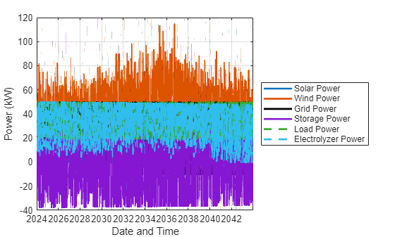
Figure contains an axes object. The axes object with xlabel Date and Time, ylabel Power (kW) contains 6 objects of type line. These objects represent Solar Power, Wind Power, Grid Power, Storage Power, Load Power, Electrolyzer Power.

要更详细地查看曲线，请放大以查看一周的时间段。

xlim([t(1e3),t(1e3+24*7)])

详细程度揭示了以下内容：

电网功率和负载功率曲线相同。在此时间范围内，负载完全由电网供电。
当太阳能接近其最大值时，存储功率趋于负值。当有太阳能时，电池系统会储存一些太阳能，而当没有太阳能时，电池系统则会提供电力。
电解槽功率与风力发电有相关，但并不完全相同。

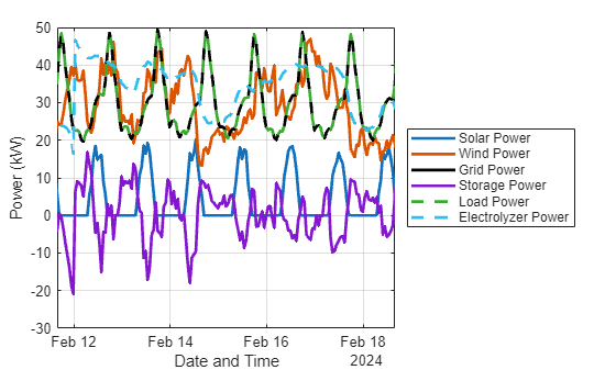
绘制电网功率和电网价格曲线。

figure
plot(t,sol.gridPower,"k");
xlabel("Date and Time"),ylabel("Grid Power (kW)")
grid
hold on
yyaxis right
plot(t,data.priceGrid);
ylabel("Grid Power Price ($/kW)")
ylim([min(data.priceGrid) max(data.priceGrid)])
hold off

Figure contains an axes object. The axes object with xlabel Date and Time, ylabel Grid Power Price ($/kW) contains 2 objects of type line.

放大以仔细观察。

xlim([t(1e5) t(1.002e5)])

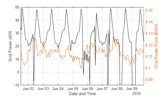
Figure contains an axes object. The axes object with xlabel Date and Time, ylabel Grid Power Price ($/kW) contains 2 objects of type line.

电网电力有时会变成负值，表示电力被卖回给电网。
当电网价格较高时，电力通常会被卖回给电网，但并非总是如此。这一结果凸显了在针对此类复杂问题做出决策时使用优化的价值。

计算并绘制累计氢气销量。

H2_sold_cum = cumsum(sol.H2_stored);
totalH2 = H2_sold_cum(end);
fprintf("Total H2 sold in kg: %g\n",totalH2)

Total H2 sold in kg: 1.09694e+07

figure
plot(t,H2_sold_cum);
xlabel("Date and Time")
ylabel("Cumulative Hydrogen Sold (kg)")
grid

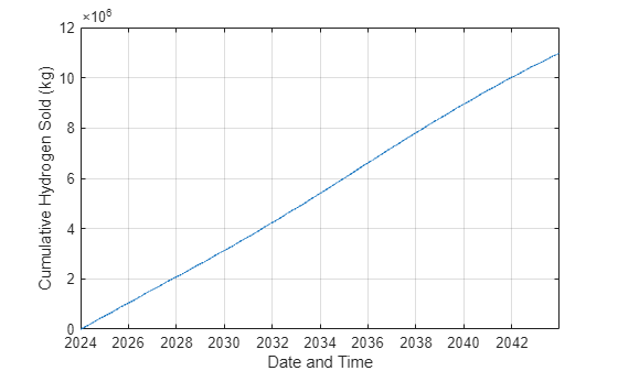
Figure contains an axes object. The axes object with xlabel Date and Time, ylabel Cumulative Hydrogen Sold (kg) contains an object of type line.

累计销售的氢气量随时间呈线性增加（大致如此）。

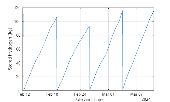
绘制四周内氢的储存分布图。请注意，储存的氢气在一周内会增加，然后在周末出售时下降。

figure
plot(t,sol.H2_stored);
xlabel("Date and Time")
ylabel("Stored Hydrogen (kg)")
xlim([t(1e3),t(1e3+24*7*4)])
grid

Figure contains an axes object. The axes object with xlabel Date and Time, ylabel Stored Hydrogen (kg) contains an object of type line.

更改折现率

折现率对于该系统的经济性有何影响？计算一系列折现率的结果。此计算需要很长时间，因此，如果可以的话，请使用并行计算。

nrates = 16;
discountRate = linspace(.02,.08,nrates);
% Create arrays to hold the results.
sols = cell(nrates,1);
fvals = zeros(1,nrates);
opt.Display = "none";
allconstraints = H2productionProblem.Constraints;
tic
parfor i = 1:nrates
    NPVCorrection = 1./((1+discountRate(i)).^(1:numYears));
    NPV = dot(H2cashFlowAnnual,NPVCorrection) - ...
        (dot(gridCashFlowAnnual,NPVCorrection) + ...
        storageEnergyRating*storageEnergyCost + ...
        storagePowerRating*storagePowerCost + ...
        storageFixedCost + ...
        solarRating*solarPowerCost + ...
        windRating*windPowerCost + ...
        electrolyzerPowerRating*electrolyzerPowerCost);
    H2productionProblem = optimproblem(Objective=NPV,...
        Constraints=allconstraints,ObjectiveSense="max");
    [tempsol,tempfval] = solve(H2productionProblem,Options=opt);
    sols{i} = tempsol;
    fvals(i) = tempfval;
end

Starting parallel pool (parpool) using the 'Processes' profile ...
Connected to parallel pool with 4 workers.

toc

Elapsed time is 2822.702064 seconds.

将 NPV 绘制为折现率的函数。

figure
plot(discountRate,fvals,"bo")
xlabel("Discount Rate")
ylabel("NPV")

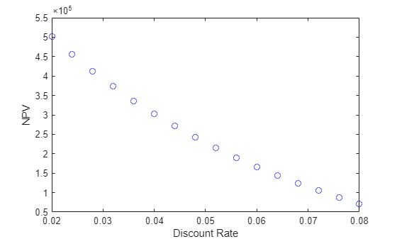
Figure contains an axes object. The axes object with xlabel Discount Rate, ylabel NPV contains a line object which displays its values using only markers.

随着折现率从 2% 增加到 8%，最佳 NPV 从 5e5 平稳下降到 7e4。最优曲线看起来是凸的，这意味着当折现率较小时，NPV 对折现率的变化更敏感，而当折现率较大时，NPV 对折现率的变化不太敏感。

绘制最佳太阳能、风能、储能和电解器额定值如何响应不同的折现率。

solarPowerRatings = zeros(1,nrates);
windPowerRatings = zeros(1,nrates);
storagePowerRatings = zeros(1,nrates);
storageEnergyRatings = zeros(1,nrates);
electrolyzerPowerRatings = zeros(1,nrates);
Total_H2_Sold = zeros(1,nrates);
for i = 1:nrates
    solarPowerRatings(i) = sols{i}.solarRating;
    windPowerRatings(i) = sols{i}.windRating;
    storagePowerRatings(i) = sols{i}.storagePowerRating;
    storageEnergyRatings(i) = sols{i}.storageEnergyRating;
    electrolyzerPowerRatings(i) = sols{i}.electrolyzerPowerRating;
    Total_H2_Sold(i) = sum(sols{i}.H2_stored);
end
figure
tiledlayout(3,2,TileSpacing="tight")
nexttile
plot(discountRate,solarPowerRatings,"bo")
xlabel("Discount Rate")
ylabel("Solar Power")
nexttile
plot(discountRate,windPowerRatings,"bo")
xlabel("Discount Rate")
ylabel("Wind Power")
nexttile
plot(discountRate,storagePowerRatings,"bo")
xlabel("Discount Rate")
ylabel("Storage Power")
nexttile
plot(discountRate,storageEnergyRatings,"bo")
xlabel("Discount Rate")
ylabel("Storage Energy")
nexttile
plot(discountRate,electrolyzerPowerRatings,"bo")
xlabel("Discount Rate")
ylabel("Electrolyzer Power")
ylim([49 50])
nexttile
plot(discountRate,Total_H2_Sold,"bo")
xlabel("Discount Rate")
ylabel("Total H2 Sold")

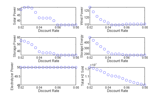
太阳能发电评级不是折现率的单调函数。观测到的最高最佳太阳能功率等级约为 52 千瓦，最小约为 36 千瓦。
同样地，风能评级对折现率也没有单调的响应。观测到的最高风力额定功率接近 128 千瓦，最低风力额定功率略高于 114 千瓦。
存储功率额定值不增加。观察到的最高存储功率额定值为 55 kW，最低为 34 kW。
同样地，存储能量等级也是不增加的。观察到的最高存储能量等级接近 500 kWh，最低存储能量等级略低于 200 kWh。
对于所有折现率来说，最佳电解器额定功率为 50 kW。这个结果意味着您可以通过使用更高的电解器功率额定值来提高 NPV。
20 年期间销售的氢气总量随折现率单调递减，既不凹也不凸。观察到的氢气销量最高为 1.2e7 公斤以上，最低为 1e7 公斤以下。

结论

绿色氢气生产系统的分析表明，该系统对于 2%至 8%之间的所有折现率都是经济的。系统的运行细节随着不同的折现率而显示出一些意想不到的变化。具体来说，系统组件评级不是折现率的严格单调函数。最佳解包括各种系统组件的每小时设置，如检查系统操作部分所示。

另请参阅

linprog | solve