绘图函数

在执行过程中对优化绘图

您可以在求解器的执行过程中绘制各种进度测度。使用 optimoptions 的 PlotFcn 名称-值参量为求解器指定一个或多个绘图函数，以在每次迭代时调用。传递函数句柄、函数名称或者由函数句柄或函数名称组成的元胞数组作为 PlotFcn 值。

每个求解器都有多个可用的预定义绘图函数。有关详细信息，请参阅求解器的函数参考页上的 PlotFcn 选项描述。

您也可以使用自定义绘图函数，如创建自定义绘图函数中所示。使用与输出函数相同的结构体编写一个函数文件。有关此结构体的详细信息，请参阅输出函数和绘图函数语法。

使用预定义的绘图函数

打开实时脚本

此示例说明如何使用绘图函数查看 fmincon "interior-point" 算法的进度。此问题取自使用优化实时编辑器任务或求解器的有约束非线性问题。

编写非线性目标函数和约束函数，包括其梯度。目标函数是罗森布罗克函数。

type rosenbrockwithgrad

function [f,g] = rosenbrockwithgrad(x)
% Calculate objective f
f = 100*(x(2) - x(1)^2)^2 + (1-x(1))^2;

if nargout > 1 % gradient required
    g = [-400*(x(2)-x(1)^2)*x(1)-2*(1-x(1));
        200*(x(2)-x(1)^2)];
end

将此文件另存为 rosenbrockwithgrad.m。

约束函数的解满足 norm(x)^2 <= 1。

type unitdisk2

function [c,ceq,gc,gceq] = unitdisk2(x)
c = x(1)^2 + x(2)^2 - 1;
ceq = [ ];

if nargout > 2
    gc = [2*x(1);2*x(2)];
    gceq = [];
end

将此文件另存为 unitdisk2.m。

为求解器创建包括调用三个绘图函数的 options 结构体。

options = optimoptions(@fmincon,Algorithm="interior-point",...
 SpecifyObjectiveGradient=true,SpecifyConstraintGradient=true,...
 PlotFcn={@optimplotx,@optimplotfval,@optimplotfirstorderopt});

创建初始点 x0 = [0,0]，并将其余输入设置为空 ([])。

x0 = [0,0];
A = [];
b = [];
Aeq = [];
beq = [];
lb = [];
ub = [];

调用 fmincon，包括选项。

fun = @rosenbrockwithgrad;
nonlcon = @unitdisk2;
x = fmincon(fun,x0,A,b,Aeq,beq,lb,ub,nonlcon,options)

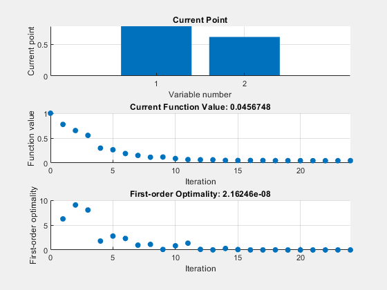
Local minimum found that satisfies the constraints.

Optimization completed because the objective function is non-decreasing in 
feasible directions, to within the value of the optimality tolerance,
and constraints are satisfied to within the value of the constraint tolerance.

<stopping criteria details>

x = 1×2

    0.7864    0.6177

创建自定义绘图函数

打开实时脚本

要为 Optimization Toolbox™ 求解器创建自定义绘图函数，请使用以下语法编写函数

function stop = plotfun(x,optimValues,state)
stop = false;
switch state
    case "init"
        % Set up plot
    case "iter"
        % Plot points
    case "done"
        % Clean up plots
    % Some solvers also use case "interrupt"
end
end

Global Optimization Toolbox 求解器使用不同语法。

软件将 x、optimValues 和 state 数据传递给绘图函数。有关完整的语法详细信息和 optimValues 参量中的数据列表，请参阅输出函数和绘图函数语法。使用 PlotFcn 名称-值参量将绘图函数名称传递给求解器。

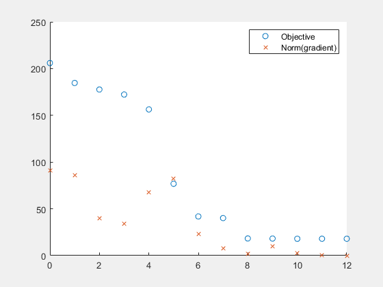
例如，在此示例末尾列出的 plotfandgrad 辅助函数绘制标量值目标函数的目标函数值和梯度范数。使用此示例末尾列出的 ras 辅助函数作为目标函数。ras 函数包括梯度计算，因此为了提高效率，请将 SpecifyObjectiveGradient 名称-值参量设置为 true。

fun = @ras;
rng(1) % For reproducibility
x0 = 10*randn(2,1); % Random initial point
opts = optimoptions(@fminunc,SpecifyObjectiveGradient=true,PlotFcn=@plotfandgrad);
[x,fval] = fminunc(fun,x0,opts)

Figure Optimization Plot Function contains an axes object. The axes object contains 2 objects of type line. One or more of the lines displays its values using only markers These objects represent Objective, Norm(gradient).

Local minimum found.

Optimization completed because the size of the gradient is less than
the value of the optimality tolerance.

<stopping criteria details>

fval = 
17.9798

绘图显示梯度的范数收敛于零，与无约束优化的预期相符。

辅助函数

以下代码会创建 plotfandgrad 辅助函数。

function stop = plotfandgrad(x,optimValues,state)
persistent iters fvals grads % Retain these values throughout the optimization
stop = false;

switch state
    case "init"
        iters = [];
        fvals = [];
        grads = [];
    case "iter"
        iters = [iters optimValues.iteration];
        fvals = [fvals optimValues.fval];
        grads = [grads norm(optimValues.gradient)];
        plot(iters,fvals,"o",iters,grads,"x");
        legend("Objective","Norm(gradient)")
    case "done"
end
end

以下代码会创建 ras 辅助函数。

function [f,g] = ras(x)
f = 20 + x(1)^2 + x(2)^2 - 10*cos(2*pi*x(1) + 2*pi*x(2));
if nargout > 1
    g(2) = 2*x(2) + 20*pi*sin(2*pi*x(1) + 2*pi*x(2));
    g(1) = 2*x(1) + 20*pi*sin(2*pi*x(1) + 2*pi*x(2));
end
end

绘图函数

在执行过程中对优化绘图

使用预定义的绘图函数

创建自定义绘图函数

另请参阅

主题