基于问题求解有约束非线性优化
此示例说明如何通过使用基于问题的方法寻找具有非线性约束的非线性目标函数的最小值。有关类似问题求解的视频,请参阅基于问题的非线性规划。
要使用基于问题的方法找到非线性目标函数的最小值,请首先将目标函数编写为文件或匿名函数。此示例的目标函数是
function f = objfunx(x,y)
f = exp(x).*(4*x.^2 + 2*y.^2 + 4*x.*y + 2*y - 1);
end
创建优化问题变量 x 和 y。
x = optimvar("x");
y = optimvar("y");
使用优化变量的表达式创建目标函数。
obj = objfunx(x,y);
创建一个以 obj 为目标函数的优化问题。
prob = optimproblem(Objective=obj);
创建一个使解位于倾斜椭圆中的非线性约束,指定为
使用优化变量的不等式表达式创建约束。
TiltEllipse = x.*y/2 + (x+2).^2 + (y-2).^2/2 <= 2;
在问题中包含该约束。
prob.Constraints.constr = TiltEllipse;
创建一个结构体,将初始点表示为 x = –3、y = 3。
x0.x = -3;
x0.y = 3;
检查此问题。
show(prob)
  OptimizationProblem :

	Solve for:
       x, y

	minimize :
       (exp(x) .* (((((4 .* x.^2) + (2 .* y.^2)) + ((4 .* x) .* y)) + (2 .* y)) - 1))


	subject to constr:
       ((((x .* y) ./ 2) + (x + 2).^2) + ((y - 2).^2 ./ 2)) <= 2
求解。
[sol,fval] = solve(prob,x0)
Solving problem using fmincon.

Local minimum found that satisfies the constraints.

Optimization completed because the objective function is non-decreasing in
feasible directions, to within the value of the optimality tolerance,
and constraints are satisfied to within the value of the constraint tolerance.

<stopping criteria details>
sol = struct with fields:
    x: -5.2813
    y: 4.6815
fval =
0.3299
尝试不同起点。
x0.x = -1;
x0.y = 1;
[sol2,fval2] = solve(prob,x0)
Solving problem using fmincon.

Feasible point with lower objective function value found, but optimality criteria not satisfied. See output.bestfeasible..


Local minimum found that satisfies the constraints.

Optimization completed because the objective function is non-decreasing in
feasible directions, to within the value of the optimality tolerance,
and constraints are satisfied to within the value of the constraint tolerance.

<stopping criteria details>
sol2 = struct with fields:
    x: -0.8210
    y: 0.6696
fval2 =
0.7626
绘制椭圆、目标函数等高线和两个解。
f = @objfunx;
g = @(x,y) x.*y/2+(x+2).^2+(y-2).^2/2-2;
rnge = [-5.5 -0.25 -0.25 7];
fimplicit(g,"k-")
axis(rnge);
hold on
fcontour(f,rnge,LevelList=logspace(-1,1))
plot(sol.x,sol.y,"ro",LineWidth=2)
plot(sol2.x,sol2.y,"ko",LineWidth=2)
legend("Constraint","f Contours","Global Solution","Local Solution",Location="northeast");
hold off
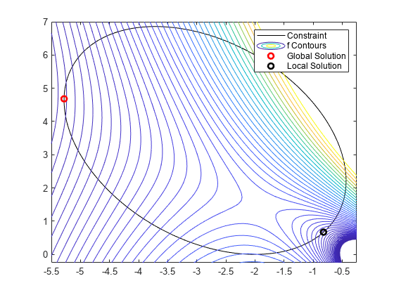
解位于非线性约束边界上。等高线图显示这些是仅有的局部最小值。该图还显示在 [–2,3/2] 附近存在一个平稳点,在 [–2,0] 和 [–1,4] 附近存在局部最大值。
使用 fcn2optimexpr 转换目标函数
对于某些目标函数或软件版本,您必须使用 fcn2optimexpr 将非线性函数转换为优化表达式。请参阅优化变量和表达式支持的运算和将非线性函数转换为优化表达式。在 fcn2optimexpr 调用中传递 x 和 y 变量,以指示每个 objfunx 输入对应的优化变量。
obj = fcn2optimexpr(@objfunx,x,y);
像前面一样,创建一个以 obj 为目标函数的优化问题。
prob = optimproblem(Objective=obj);
求解过程的其余部分是相同的。