使用大型计算集群分析风能数据
此示例展示了如何访问云中的大型数据集并使用大型集群上的数百个工作单元对其进行处理。
在此示例中,您使用数据存储和 Parallel Computing Toolbox™ 对美国大陆超过 120,000 个站点进行风能资源评估研究,以确定最适合建设风电场的最佳地点。
本示例中的公共数据集是 Wind Integration 国家数据集工具包(或 WIND 工具包 [1]、[2]、[3]、[4])的一部分。欲了解更多信息,请参阅风能集成国家数据集工具包。WIND 工具包存储在被授权公开访问的公共 Amazon S3™ 存储桶中,因此您无需配置身份验证。为了获得最佳效果,请从 Amazon® Web Service (AWS®) 云集群运行此示例。
要访问远程输入数据,您必须使用环境变量指定存储桶的地理区域。
setenv("AWS_DEFAULT_REGION","us-west-2");
创建一个并行池,并将工作单元所需的函数文件附加到该池中。将客户端环境变量发送给工作单元。
numWorkers = 450;
c = parcluster("HPCProfile");
pool = parpool(c,numWorkers,EnvironmentVariables="AWS_DEFAULT_REGION", ...
    AttachedFiles=["windNCReader.m","findWindTurbineSite.m",mfilename("fullpath")]);
Starting parallel pool (parpool) using the 'HPCProfile' profile ...
Connected to parallel pool with 450 workers.
使用 FileDatastore 来管理对远程 WIND 数据集的访问。
为了加快此示例的速度,请加载预先准备的 windSitesDs 数据存储。如果您需要重新创建数据存储对象,您可以使用本示例附带的 createWindSitesDatastore 辅助函数。
load("windSitesDs.mat","windSitesDs")
% windSitesDs = createWindSitesDatastore;
检查工作单元是否可以访问 S3 存储桶中的文件,然后重置数据存储。
f = parfeval(@(ds) summary(read(ds)),1,windSitesDs);
testOut = fetchOutputs(f)
testOut = struct with fields:
              Time: [1×1 struct]
        wind_speed: [1×1 struct]
    wind_direction: [1×1 struct]
           density: [1×1 struct]
       temperature: [1×1 struct]
          pressure: [1×1 struct]
reset(windSitesDs);
处理站点数据
准备地理散点图来跟踪计算
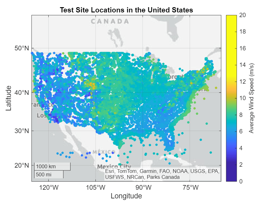
预先分配一个表来收集进度摘要。initializeGeoScatter 辅助函数初始化地理散点图以可视化不同的测试位置并准备标题、标签和限制等设置。
itbl = table(size=[0,5],VariableTypes=["single","string","single","single","single"], ...
    VariableNames=["SiteID","ValueStoreKey","Latitude","Longitude","AvgWindSpeed"]);
s = initializeGeoScatter(itbl);
设置 DataQueue 来跟踪进度
创建一个 DataQueue 对象,用于将进度摘要从工作单元发送到客户端。使用 afterEach 函数在客户端上定义一个回调,每次工作单元发送计算进度时更新地理散点图。
d = parallel.pool.DataQueue;
afterEach(d,@(x) updateGeoPlot(s,x));
执行计算并更新进度
准备一个 parfor 循环来独立处理数据存储中的文件。
在 parfor 循环内,根据并行池中工作单元的数量对数据存储进行分区。初始化一个元胞数组来存储进度数据,并指定在工作单元将进度数据发送到客户端之前要处理的文件数量。然后,使用此示例附带的 findWindTurbine 辅助函数读取并分析数据存储中每个文件的数据。
np = numpartitions(windSitesDs,pool);
parfor a = 1:np
    ds = partition(windSitesDs,np,a);
    updateSize = 12;
    geoTblUpdate = cell(updateSize,5);
    store = getCurrentValueStore;
    count = 0
    updateCount = 0

    while hasdata(ds)
        count = count+1;
        updateCount = updateCount+1;
        t = read(ds);
        results = findWindTurbineSite(t);
将结果存储在池的 ValueStore 对象中。当所有结果的总和很大时,或者客户端在 ValueStore 循环期间需要结果时,可以使用 parfor-。否则,如果您的数据很小或不需要在 parfor 代码块内,则 parfor 输出通常会提供更快的性能。
        key = strcat("set_",num2str(a)," result_",num2str(count));
        store(key) = results;
收集每次迭代的进度摘要。
        geoTblUpdate(updateCount,:) = {results.siteMetadata.siteID, ...
            key, ...
            results.siteMetadata.latitude, ...
            results.siteMetadata.longitude, ...
            results.overallData.wind_speed.Avg};
您可以指定将数据发送回客户端的频率。处理完 12 个文件后,将收集到的现场信息和初步结果发送给客户端。
        if updateCount >= updateSize
            send(d,geoTblUpdate);
            updateCount = 0;
            geoTblUpdate = cell(updateSize,5);
        end
    end
    if updateCount > 0
        send(d,geoTblUpdate(1:updateCount,:));
        updateCount = 0;
        geoTblUpdate = {};
    end
end
执行后处理分析
您现在可以以交互方式访问池的 ValueStore 中的结果。在此示例中,使用 ValueStore 是有效的,因为您将数据保留在集群存储上,直到删除并行池。这样就无需在后期数据分析期间与客户端之间传输数据。此类传输可能会产生数据开销,尤其是在数据量巨大或网络高延迟下。
使用另一个 parfor 循环执行后分析缩减操作以找到产生最大功率的站点。
clientStore = pool.ValueStore;
keySet = keys(clientStore);
maxPowerAndKey = cell(1,2);
parfor k = 1:length(keySet)
    store = getCurrentValueStore;
    key = keySet(k);
    results = store(key);
    maxPower = results.powerResults.maxPower;
    maxPowerAndKey = compareValue(maxPowerAndKey,{maxPower,key});
end
disp(maxPowerAndKey)
{[1.5374]} {["set_1534 result_5"]}
key = maxPowerAndKey{2};
bestSite = clientStore(key);
有前景的网站统计摘要
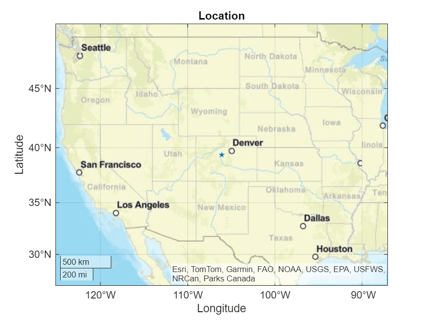
查看对风力发电场最佳场址预测的摘要。
站点信息
fprintf("Site ID: %d",bestSite.siteMetadata.siteID)Site ID: 47084
figure;
geoscatter(bestSite.siteMetadata.latitude,bestSite.siteMetadata.longitude,"pentagram","filled");
title("Location")
geobasemap streets
风力统计信息
fprintf("Mean Wind Speed (m/s): %3.2f\n" + ...
    "Std. Dev. of Wind Speed (m/s): %3.2f\n" + ...
    "Max. Wind Speed (m/s): %3.2f\n", ...
    bestSite.overallData.wind_speed.Avg,bestSite.overallData.wind_speed.StdDev,bestSite.overallData.wind_speed.Max);
Mean Wind Speed (m/s): 11.56
Std. Dev. of Wind Speed (m/s): 5.06
Max. Wind Speed (m/s): 36.73
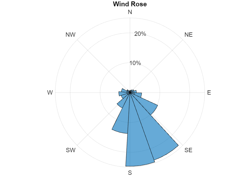
在风玫瑰图中显示风向分布。
figure;
h = polarhistogram("BinEdge",bestSite.windDirectionHist.edges,"BinCounts",bestSite.windDirectionHist.counts);
pax = gca;
pax.ThetaZeroLocation = "top";
pax.ThetaDir = 'clockwise';
pax.ThetaTick = 0:45:360;
pax.ThetaTickLabel = ["N","NE","E","SE","S","SW","W","NW"];
pax.RTickLabel = num2str(str2double(pax.RTickLabel)*100)+"%";
title("Wind Rose")
显示每种风力涡轮机的年功率、容量系数和年能量产量的摘要。
disp(bestSite.powerResults.summary)
    Turbine Class    Turbine Rated Power (MW)    Averaged Power (kW)    Capacity Factor (%)    Annual Energy Production (MWh)
    _____________    ________________________    ___________________    ___________________    ______________________________

          1                     2                      1443.4                 72.171                       12644
          2                     2                      1537.4                 76.871                       13468
          3                     2                      1518.2                 75.911                       13300
分析完结果数据后,您可以删除并行池。删除并行池也会删除 ValueStore 中的数据,因此如果您想保留数据,请在删除池之前将 ValueStore 中的数据复制到另一个位置。
delete(pool);
局部函数
initializeGeoScatter 函数初始化一个地理散点图,用于显示来自工作单元的更新。
function s = initializeGeoScatter(itbl)
    s = geoscatter(itbl,"Latitude","Longitude",ColorVariable="AvgWindSpeed",SizeData=10,MarkerFaceColor="flat");
    c = colorbar;
    c.Label.String = "Average Wind Speed (m/s)";
    c.Limits = [0,20];
    title("Test Site Locations in the United States");
    geolimits([25 50],[-125.4 -65.0]);
end
compareValue 函数确定两个输入元胞数组中的哪一个在第一个位置包含较大的数值,并返回相应的元胞数组。
function v = compareValue(currentMaxPower,candidate)
    valueA = currentMaxPower{1};
    valueB = candidate{1};
    if valueA > valueB
        v = currentMaxPower;
    else
        v = candidate;
    end
end
当工作单元向客户端发送新数据时,updateGeoPlot 函数会更新地理散点图。
function updateGeoPlot(s,x)
    s.SourceTable = [s.SourceTable;x];
    drawnow limitrate nocallbacks;
end
参考资料
[1] Draxl, Caroline, Bri-Mathias Hodge, Andrew Clifton, and Jim McCaa."Overview and Meteorological Validation of the Wind Integration National Dataset Toolkit (Technical Report, NREL/TP-5000-61740)".Golden, CO:National Renewable Energy Laboratory (2015). https://www.nrel.gov/docs/fy15osti/61740.pdf
[2] Draxl, Caroline, Andrew Clifton, Bri-Mathias Hodge, and Jim McCaa.“The Wind Integration National Dataset (WIND) Toolkit.”Applied Energy 151 (August 2015):355–66 https://doi.org/10.1016/j.apenergy.2015.03.121
[3] King, J., Andrew Clifton, and Bri-Mathias Hodge."Validation of Power Output for the WIND Toolkit (Technical Report, NREL/TP-5D00-61714)".Golden, CO:National Renewable Energy Laboratory (2014). https://www.nrel.gov/docs/fy14osti/61714.pdf
[4] Lieberman-Cribbin, W., Caroline Draxl, and Andrew Clifton."Guide to Using the WIND Toolkit Validation Code (Technical Report, NREL/TP-5000-62595)".Golden, CO:National Renewable Energy Laboratory (2014). https://www.nrel.gov/docs/fy15osti/62595.pdf
[5] “WTK_Validation_IEC-1_normalized - NREL/Turbine-Models Power Curve Archive 0 Documentation.”Accessed December 5, 2023. https://nrel.github.io/turbine-models/WTK_Validation_IEC-1_normalized.html
[6] “WTK_Validation_IEC-2_normalized - NREL/Turbine-Models Power Curve Archive 0 Documentation.”Accessed December 5, 2023. https://nrel.github.io/turbine-models/WTK_Validation_IEC-2_normalized.html
[7] “WTK_Validation_IEC-3_normalized - NREL/Turbine-Models Power Curve Archive 0 Documentation.”Accessed December 5, 2023. https://nrel.github.io/turbine-models/WTK_Validation_IEC-3_normalized.html