在 GPU 上对 A\b 进行基准测试
这个示例研究如何在 GPU 上对线性系统的求解进行基准测试。用于解决 x 中的 A*x = b 的 MATLAB® 代码非常简单。最常见的是,我们使用矩阵左除法(也称为 mldivide 或反斜杠运算符 (\) 来计算 x(即 x = A\b)。
相关示例:
基准测试 A\ b 使用分布式数组。
本示例中显示的代码可以在以下函数中找到:
function results = paralleldemo_gpu_backslash(maxMemory)
选择适合计算的矩阵大小非常重要。我们可以通过指定 CPU 和 GPU 可用的系统内存量(以 GB 为单位)来实现这一点。默认值仅基于 GPU 上可用的内存量,您可以指定适合您系统的值。
if nargin == 0
    g = gpuDevice;
    maxMemory = 0.4*g.AvailableMemory/1024^3;
end
基准测试函数
我们希望对矩阵左除法 (\) 进行基准测试,而不是对 CPU 和 GPU 之间传输数据的成本、创建矩阵所需的时间或其他参数进行基准测试。因此,我们将数据生成与线性系统的求解分开,只测量后者所需的时间。
function [A, b] = getData(n, clz)
    fprintf('Creating a matrix of size %d-by-%d.\n', n, n);
    A = rand(n, n, clz) + 100*eye(n, n, clz);
    b = rand(n, 1, clz);
end

function time = timeSolve(A, b, waitFcn)
    tic;
    x = A\b; %#ok<NASGU> We don't need the value of x.
    waitFcn(); % Wait for operation to complete.
    time = toc;
end
选择问题大小
与许多其他并行算法一样,并行求解线性系统的性能很大程度上取决于矩阵大小。如在其他示例中所见,例如基准测试 A\ b,我们比较了不同矩阵大小的算法的性能。
% Declare the matrix sizes to be a multiple of 1024.
maxSizeSingle = floor(sqrt(maxMemory*1024^3/4));
maxSizeDouble = floor(sqrt(maxMemory*1024^3/8));
step = 1024;
if maxSizeDouble/step >= 10
    step = step*floor(maxSizeDouble/(5*step));
end
sizeSingle = 1024:step:maxSizeSingle;
sizeDouble = 1024:step:maxSizeDouble;
比较性能:Gigaflops
我们使用每秒浮点运算次数作为性能衡量标准,因为这使我们能够比较不同矩阵大小的算法的性能。
给定一个矩阵大小,基准测试函数会创建矩阵 A 和右侧 b 一次,然后求解 A\b 几次以准确测量所需时间。我们使用 HPC Challenge 的浮点运算计数,因此对于 n×n 矩阵,我们将浮点运算计为 2/3*n^3 + 3/2*n^2。
该函数通过句柄传递给“等待”函数。在 CPU 上,此函数不执行任何操作。在 GPU 上,此函数等待所有待处理的操作完成。以这种方式等待可确保准确的时间。
function gflops = benchFcn(A, b, waitFcn)
    numReps = 3;
    time = inf;
    % We solve the linear system a few times and calculate the Gigaflops
    % based on the best time.
    for itr = 1:numReps
        tcurr = timeSolve(A, b, waitFcn);
        time = min(tcurr, time);
    end

    % Measure the overhead introduced by calling the wait function.
    tover = inf;
    for itr = 1:numReps
        tic;
        waitFcn();
        tcurr = toc;
        tover = min(tcurr, tover);
    end
    % Remove the overhead from the measured time. Don't allow the time to
    % become negative.
    time = max(time - tover, 0);
    n = size(A, 1);
    flop = 2/3*n^3 + 3/2*n^2;
    gflops = flop/time/1e9;
end

% The CPU doesn't need to wait: this function handle is a placeholder.
function waitForCpu()
end

% On the GPU, to ensure accurate timing, we need to wait for the device
% to finish all pending operations.
function waitForGpu(theDevice)
    wait(theDevice);
end
执行基准测试
完成所有设置后,执行基准测试就很简单了。然而,计算可能需要很长时间才能完成,因此我们在完成每个矩阵大小的基准测试时打印一些中间状态信息。我们还将遍历所有矩阵大小的循环封装在一个函数中,以对单精度和双精度计算进行基准测试。
function [gflopsCPU, gflopsGPU] = executeBenchmarks(clz, sizes)
    fprintf(['Starting benchmarks with %d different %s-precision ' ...
         'matrices of sizes\nranging from %d-by-%d to %d-by-%d.\n'], ...
            length(sizes), clz, sizes(1), sizes(1), sizes(end), ...
            sizes(end));
    gflopsGPU = zeros(size(sizes));
    gflopsCPU = zeros(size(sizes));
    gd = gpuDevice;
    for i = 1:length(sizes)
        n = sizes(i);
        [A, b] = getData(n, clz);
        gflopsCPU(i) = benchFcn(A, b, @waitForCpu);
        fprintf('Gigaflops on CPU: %f\n', gflopsCPU(i));
        A = gpuArray(A);
        b = gpuArray(b);
        gflopsGPU(i) = benchFcn(A, b, @() waitForGpu(gd));
        fprintf('Gigaflops on GPU: %f\n', gflopsGPU(i));
    end
end
然后我们以单精度和双精度执行基准测试。
[cpu, gpu] = executeBenchmarks('single', sizeSingle);
results.sizeSingle = sizeSingle;
results.gflopsSingleCPU = cpu;
results.gflopsSingleGPU = gpu;
[cpu, gpu] = executeBenchmarks('double', sizeDouble);
results.sizeDouble = sizeDouble;
results.gflopsDoubleCPU = cpu;
results.gflopsDoubleGPU = gpu;
Starting benchmarks with 7 different single-precision matrices of sizes
ranging from 1024-by-1024 to 19456-by-19456.
Creating a matrix of size 1024-by-1024.
Gigaflops on CPU: 43.805496
Gigaflops on GPU: 78.474002
Creating a matrix of size 4096-by-4096.
Gigaflops on CPU: 96.459635
Gigaflops on GPU: 573.278854
Creating a matrix of size 7168-by-7168.
Gigaflops on CPU: 184.997657
Gigaflops on GPU: 862.755636
Creating a matrix of size 10240-by-10240.
Gigaflops on CPU: 204.404384
Gigaflops on GPU: 978.362901
Creating a matrix of size 13312-by-13312.
Gigaflops on CPU: 218.773070
Gigaflops on GPU: 1107.983667
Creating a matrix of size 16384-by-16384.
Gigaflops on CPU: 233.529176
Gigaflops on GPU: 1186.423754
Creating a matrix of size 19456-by-19456.
Gigaflops on CPU: 241.482550
Gigaflops on GPU: 1199.151846
Starting benchmarks with 5 different double-precision matrices of sizes
ranging from 1024-by-1024 to 13312-by-13312.
Creating a matrix of size 1024-by-1024.
Gigaflops on CPU: 34.902918
Gigaflops on GPU: 72.191488
Creating a matrix of size 4096-by-4096.
Gigaflops on CPU: 74.458136
Gigaflops on GPU: 365.339897
Creating a matrix of size 7168-by-7168.
Gigaflops on CPU: 93.313782
Gigaflops on GPU: 522.514165
Creating a matrix of size 10240-by-10240.
Gigaflops on CPU: 104.219804
Gigaflops on GPU: 628.301313
Creating a matrix of size 13312-by-13312.
Gigaflops on CPU: 108.826886
Gigaflops on GPU: 681.881032
绘制性能图
我们现在可以绘制结果,并比较 CPU 和 GPU 上的单精度和双精度性能。
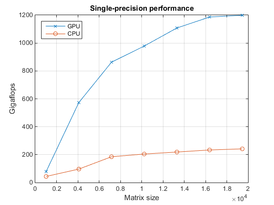
首先,我们看一下单精度反斜杠运算符的性能。
fig = figure;
ax = axes('parent', fig);
plot(ax, results.sizeSingle, results.gflopsSingleGPU, '-x', ...
     results.sizeSingle, results.gflopsSingleCPU, '-o')
grid on;
legend('GPU', 'CPU', 'Location', 'NorthWest');
title(ax, 'Single-precision performance')
ylabel(ax, 'Gigaflops');
xlabel(ax, 'Matrix size');
drawnow;
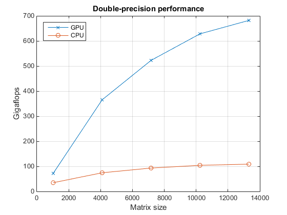
现在,我们来看看双精度反斜杠运算符的性能。
fig = figure;
ax = axes('parent', fig);
plot(ax, results.sizeDouble, results.gflopsDoubleGPU, '-x', ...
     results.sizeDouble, results.gflopsDoubleCPU, '-o')
legend('GPU', 'CPU', 'Location', 'NorthWest');
grid on;
title(ax, 'Double-precision performance')
ylabel(ax, 'Gigaflops');
xlabel(ax, 'Matrix size');
drawnow;
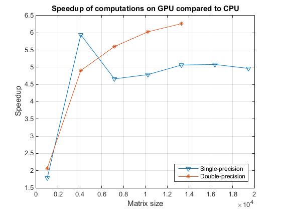
最后,我们来比较一下 GPU 与 CPU 之间反斜杠运算符的加速情况。
speedupDouble = results.gflopsDoubleGPU./results.gflopsDoubleCPU;
speedupSingle = results.gflopsSingleGPU./results.gflopsSingleCPU;
fig = figure;
ax = axes('parent', fig);
plot(ax, results.sizeSingle, speedupSingle, '-v', ...
     results.sizeDouble, speedupDouble, '-*')
grid on;
legend('Single-precision', 'Double-precision', 'Location', 'SouthEast');
title(ax, 'Speedup of computations on GPU compared to CPU');
ylabel(ax, 'Speedup');
xlabel(ax, 'Matrix size');
drawnow;
end
ans =

         sizeSingle: [1024 4096 7168 10240 13312 16384 19456]
    gflopsSingleCPU: [1x7 double]
    gflopsSingleGPU: [1x7 double]
         sizeDouble: [1024 4096 7168 10240 13312]
    gflopsDoubleCPU: [34.9029 74.4581 93.3138 104.2198 108.8269]
    gflopsDoubleGPU: [72.1915 365.3399 522.5142 628.3013 681.8810]
另请参阅
gpuArray | gpuDevice | mldivide