本页面提供的是上一版软件的文档。当前版本中已删除对应的英文页面。
对集群上的独立作业进行基准测试
在这个示例中,我们展示了如何使用集群上的独立作业对应用程序进行基准测试,并对结果进行了详细分析。具体来说,我们:
展示如何对顺序代码和任务并行代码的混合进行基准测试。
解释强扩展和弱扩展。
讨论客户端和集群上的一些潜在瓶颈。
注意:如果在大型集群上运行此示例,则可能需要一个小时才能运行。
相关示例:
本示例中显示的代码可以在以下函数中找到:
function paralleldemo_distribjob_bench
检查集群配置文件
在与集群交互之前,我们验证 MATLAB® 客户端是否根据我们的需求进行了配置。调用 parcluster 将为我们提供一个使用默认配置文件的集群,如果默认值不可用,则会引发错误。
myCluster = parcluster;
计时
我们对所有操作分别计时,以便我们能够详细检查它们。我们需要所有这些详细的时间来了解时间花在了哪里,并隔离潜在的瓶颈。就示例而言,我们基准测试的实际函数并不十分重要;在本示例中,我们仿真纸牌游戏二十一点或 21 点。
我们编写的所有操作都尽可能地高效。例如,我们使用向量化任务创建。我们使用 tic 和 toc 来测量所有操作的经过时间,而不是使用作业和任务属性 CreateDateTime、StartDateTime、FinishDateTime 等,因为 tic 和 toc 为我们提供了亚秒级的粒度。请注意,我们还对任务函数进行了检测,以便它返回执行基准计算所花费的时间。
function [times, description] = timeJob(myCluster, numTasks, numHands)
    % The code that creates the job and its tasks executes sequentially in
    % the MATLAB client starts here.
    % We first measure how long it takes to create a job.
    timingStart = tic;
    start = tic;
    job = createJob(myCluster);
    times.jobCreateTime = toc(start);
    description.jobCreateTime = 'Job creation time';

    % Create all the tasks in one call to createTask, and measure how long
    % that takes.
    start = tic;
    taskArgs = repmat({{numHands, 1}}, numTasks, 1);
    createTask(job, @pctdemo_task_blackjack, 2, taskArgs);
    times.taskCreateTime = toc(start);
    description.taskCreateTime = 'Task creation time';

    % Measure how long it takes to submit the job to the cluster.
    start = tic;
    submit(job);
    times.submitTime = toc(start);
    description.submitTime = 'Job submission time';

    % Once the job has been submitted, we hope all its tasks execute in
    % parallel.  We measure how long it takes for all the tasks to start
    % and to run to completion.
    start = tic;
    wait(job);
    times.jobWaitTime = toc(start);
    description.jobWaitTime = 'Job wait time';

    % Tasks have now completed, so we are again executing sequential code
    % in the MATLAB client.  We measure how long it takes to retrieve all
    % the job results.
    start = tic;
    results = fetchOutputs(job);
    times.resultsTime = toc(start);
    description.resultsTime = 'Result retrieval time';

    % Verify that the job ran without any errors.
    if ~isempty([job.Tasks.Error])
        taskErrorMsgs = pctdemo_helper_getUniqueErrors(job);
        delete(job);
        error('pctexample:distribjobbench:JobErrored',  ...
          ['The following error(s) occurred during task ' ...
          'execution:\n\n%s'], taskErrorMsgs);
    end

    % Get the execution time of the tasks.  Our task function returns this
    % as its second output argument.
    times.exeTime = max([results{:,2}]);
    description.exeTime = 'Task execution time';

    % Measure how long it takes to delete the job and all its tasks.
    start = tic;
    delete(job);
    times.deleteTime = toc(start);
    description.deleteTime = 'Job deletion time';

    % Measure the total time elapsed from creating the job up to this
    % point.
    times.totalTime = toc(timingStart);
    description.totalTime = 'Total time';

    times.numTasks = numTasks;
    description.numTasks = 'Number of tasks';
end
我们来看看我们正在测量的一些细节:
作业创建时间:創建一個作业所花的时间。对于 MATLAB 作业调度器集群,这涉及远程调用,并且 MATLAB 作业调度器在其数据库中分配空间。对于其他集群类型,作业创建涉及将一些文件写入磁盘。
任务创建时间:创建和保存任务信息所需的时间。MATLAB 作业调度器将其保存在其数据库中,而其他集群类型将其保存在文件系统上的文件中。
作业提交时间:提交作业花的时间。对于 MATLAB 作业调度器集群,我们告诉它开始执行其数据库中的作业。我们要求其他集群类型执行我们创建的所有任务。
作业等待时间:从作业提交到作业完成为止我们等待的时间。这包括从作业提交到作业完成之间发生的所有活动,比如:集群可能需要启动所有工作单元,并向工作单元发送任务信息;工作单元读取任务信息,并执行任务函数。对于 MATLAB 作业调度器集群,工作单元会将任务结果发送到 MATLAB 作业调度器,后者会将其写入其数据库,而对于其他集群类型,工作单元会将任务结果写入磁盘。
任务执行时间:仿真二十一点所花费的时间。我们对任务函数进行检测,以准确测量这个时间。这个时间也包含在作业等待时间中。
结果检索时间:将作业结果带入 MATLAB 客户端所需的时间。对于 MATLAB 作业调度器,我们从其数据库中获取它们。对于其他集群类型,我们从文件系统读取它们。
作业删除时间:删除所有作业和任务信息所需的时间。MATLAB 作业调度器将其从其数据库中删除。对于其他集群类型,我们从文件系统中删除文件。
总时间:完成上述所有操作所需的时间。
选择问题大小
我们知道大多数集群都是为批量执行中期或长期运行的作业而设计的,因此我们特意尝试让我们的基准计算落在该范围内。然而,我们不希望这个示例花费几个小时来运行,所以我们选择的问题规模使得每个任务在我们的硬件上大约需要 1 分钟,然后我们重复时间测量几次以提高准确性。根据经验,如果任务中的计算时间远远少于一分钟,那么您应该考虑 parfor 是否比作业和任务更好地满足您的低延迟需求。
numHands = 1.2e6;
numReps = 5;
我们通过运行不同数量的工作单元来探索加速,从 1、2、4、8、16 等开始,到尽可能多地使用工作单元结束。在这个示例中,我们假设我们有专门访问集群的权限来进行基准测试,并且集群的 NumWorkers 属性已经正确设置。假设情况确实如此,每个任务将立即在专用的工作单元上执行,因此我们可以将提交的任务数量与执行这些任务的工作单元数量相等。
numWorkers = myCluster.NumWorkers ;
if isinf(numWorkers) || (numWorkers == 0)
    error('pctexample:distribjobbench:InvalidNumWorkers', ...
          ['Cannot deduce the number of workers from the cluster.  ' ...
           'Set the NumWorkers on your default profile to be ' ...
           'a value other than 0 or inf.']);
end

numTasks = [pow2(0:ceil(log2(numWorkers) - 1)), numWorkers];
弱扩展测量
我们改变作业中的任务数量,并让每个任务执行固定量的工作。这被称为弱扩展,也是我们最关心的,因为我们通常会扩展到集群来解决更大的问题。应该将其与本示例后面显示的强扩展基准进行比较。基于弱扩展的加速也称为扩展加速。
fprintf(['Starting weak scaling timing.  ' ...
         'Submitting a total of %d jobs.\n'], numReps*length(numTasks));
for j = 1:length(numTasks)
    n = numTasks(j);
    for itr = 1:numReps
        [rep(itr), description] = timeJob(myCluster, n, numHands);  %#ok<AGROW>
    end
    % Retain the iteration with the lowest total time.
    totalTime = [rep.totalTime];
    fastest = find(totalTime == min(totalTime), 1);
    weak(j) = rep(fastest);  %#ok<AGROW>
    fprintf('Job wait time with %d task(s): %f seconds\n', ...
            n, weak(j).jobWaitTime);
end
Starting weak scaling timing.  Submitting a total of 45 jobs.
Job wait time with 1 task(s): 59.631733 seconds
Job wait time with 2 task(s): 60.717059 seconds
Job wait time with 4 task(s): 61.343568 seconds
Job wait time with 8 task(s): 60.759119 seconds
Job wait time with 16 task(s): 63.016560 seconds
Job wait time with 32 task(s): 64.615484 seconds
Job wait time with 64 task(s): 66.581806 seconds
Job wait time with 128 task(s): 91.043285 seconds
Job wait time with 256 task(s): 150.411704 seconds
顺序执行
我们测量计算的连续执行时间。请注意,只有具有相同的硬件和软件配置时,才应将此时间与集群上的执行时间进行比较。
seqTime = inf;
for itr = 1:numReps
    start = tic;
    pctdemo_task_blackjack(numHands, 1);
    seqTime = min(seqTime, toc(start));
end
fprintf('Sequential execution time: %f seconds\n', seqTime);
Sequential execution time: 84.771630 seconds
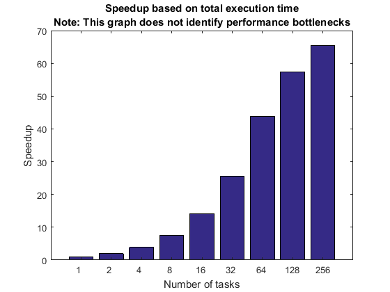
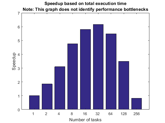
基于弱扩展和总执行时间的加速
我们首先看一下通过运行不同数量的工作单元所实现的总体加速。加速基于计算所使用的总时间,因此它包括代码的顺序部分和并行部分。
该加速曲线表示多个项目的能力,每个项目相关的权重未知:集群硬件、集群软件、客户端硬件、客户端软件以及客户端与集群之间的连接。因此,加速曲线并不代表其中任何一个,而是代表所有这些的总和。
如果加速曲线满足您期望的性能目标,您就会知道所有上述因素在这个特定的基准测试中协同作用很好。然而,如果加速曲线未能达到您的目标,您就不知道上面列出的众多因素中哪一个是主要原因。甚至可能是应用程序并行化所采用的方法有问题,而不是其他软件或硬件有问题。
新手往往认为这张图就能完整反映出他们的集群硬件或软件的性能。事实并非如此,而且我们始终需要意识到,该图不允许我们得出有关潜在性能瓶颈的任何结论。
titleStr = sprintf(['Speedup based on total execution time\n' ...
                    'Note: This graph does not identify performance ' ...
                    'bottlenecks']);
pctdemo_plot_distribjob('speedup', [weak.numTasks], [weak.totalTime], ...
    weak(1).totalTime, titleStr);
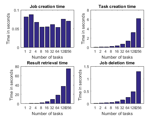
详细图,第 1 部分
我们深入挖掘一下,看看代码各个步骤所花费的时间。我们对弱扩展进行了基准测试,也就是说,我们创建的任务越多,我们执行的工作就越多。因此,随着任务数量的增加,任务输出数据的大小也会增加。考虑到这一点,我们预计创建的任务越多,以下操作花费的时间就越长:
任务创建
检索作业输出参量
作业销毁时间
我们没有理由相信以下内容会随着任务数量的增加而增加:
作业创建时间
毕竟,作业是在我们定义任何任务之前创建的,因此没有理由让它随着任务数量而变化。我们可能预计只会看到作业创造时间的一些随机波动。
pctdemo_plot_distribjob('fields', weak, description, ...
    {'jobCreateTime', 'taskCreateTime',  'resultsTime', 'deleteTime'}, ...
    'Time in seconds');
归一化时间
我们已经得出结论,随着任务数量的增加,任务创建时间预计会增加,检索作业输出参量和删除作业的时间也会增加。然而,这种增长是由于我们随着工作单元/任务数量的增加而完成了更多的工作。因此,通过查看执行这些操作所需的时间来衡量这三个活动的效率并根据任务数量对其进行标准化是有意义的。这样,我们可以观察随着任务数量的变化,以下时间是否保持不变、增加或减少:
创建单个任务所需的时间
从单个任务检索输出参量所需的时间
删除作业中的任务所需的时间
该图中的标准化时间代表 MATLAB 客户端的功能以及它可能与之交互的集群硬件或软件部分。如果这些曲线保持平坦,则通常被认为是好的,如果它们下降,则被认为是优秀的。
pctdemo_plot_distribjob('normalizedFields', weak, description, ...
    {'taskCreateTime', 'resultsTime', 'deleteTime'});
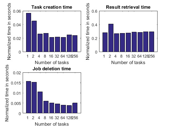
这些图有时显示,随着任务数量的增加,检索每个任务结果所花费的时间会减少。不可否认,这是件好事:我们完成的工作越多,我们的效率就越高。如果操作的开销量是固定的,并且作业中每个任务花费的时间是固定的,则可能会发生这种情况。
如果基于总执行时间的加速曲线包含大量花费在上述连续活动上的时间,并且花费的时间随着任务数量的增加而增加,那么我们就不能期望它看起来特别好。在这种情况下,一旦有足够多的任务,连续的活动就会占据主导地位。
详细图,第 2 部分
以下每个步骤所花费的时间可能会随着任务的数量而变化,但我们希望不会这样:
作业提交时间。
任务执行时间。这记录了仿真二十一点所花费的时间。不多也不少。
在这两种情况下,我们都会查看经过的时间,也称为挂钟时间。我们既不关注集群上的总 CPU 时间,也不关注标准化时间。
pctdemo_plot_distribjob('fields', weak, description, ...
    {'submitTime', 'exeTime'});
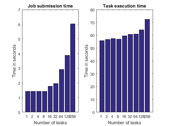
在某些情况下,上面显示的每个时间可能会随着任务数量的增加而增加。例如:
对于某些第三方集群类型,作业提交涉及作业中每个任务的一个系统调用,或者作业提交涉及通过网络复制文件。在这些情况下,作业提交时间可能会随着任务数量线性增加。
任务执行时间图最有可能暴露硬件限制和资源争用。例如,如果我们在同一台计算机上执行多个工作单元,由于对有限内存带宽的争用,任务执行时间可能会增加。资源争用的另一个示例是,如果任务函数使用单个共享文件系统读取或写入大型数据文件。然而,本示例中的任务函数根本不访问文件系统。示例 任务并行问题中的资源争用 中详细介绍了这些类型的硬件限制。
基于弱扩展和作业等待时间的加速
现在我们已经分析了代码各个阶段所花费的时间,我们希望创建一个更准确地反映集群硬件和软件功能的加速曲线。我们通过根据作业等待时间计算加速曲线来实现这一点。
在根据作业等待时间计算这个加速曲线时,我们首先将其与集群上单个任务执行作业所需的时间进行比较。
titleStr = 'Speedup based on job wait time compared to one task';
pctdemo_plot_distribjob('speedup', [weak.numTasks], [weak.jobWaitTime], ...
    weak(1).jobWaitTime, titleStr);
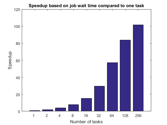
作业等待时间可能包括启动所有 MATLAB 工作单元的时间。因此,这个时间可能受到共享文件系统的 IO 功能的限制。作业等待时间还包括平均任务执行时间,因此在那里看到的任何缺陷也适用于此。如果我们没有对集群的专用访问权限,我们可以预计基于作业等待时间的加速曲线将受到严重影响。
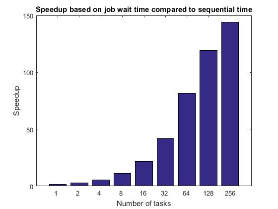
接下来,我们将作业等待时间与连续执行时间进行比较,假设客户端计算机的硬件与计算节点相当。如果客户端与集群节点没有可比性,那么这种比较是绝对没有意义的。如果您的集群在向工作单元分配任务时存在相当大的时间滞后(例如,每分钟仅向工作单元分配一次任务),则该图将受到严重影响,因为连续执行时间不会受到这种滞后的影响。请注意,该图的形状与前一个图相同,它们仅在常数乘法因子上有所不同。
titleStr = 'Speedup based on job wait time compared to sequential time';
pctdemo_plot_distribjob('speedup', [weak.numTasks], [weak.jobWaitTime], ...
    seqTime, titleStr);
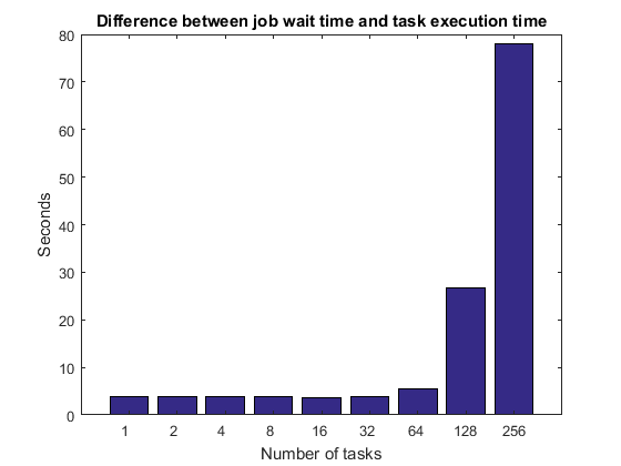
比较作业等待时间与任务执行时间
正如我们之前提到的,作业等待时间由任务执行时间加上调度、集群队列中的等待时间、MATLAB 启动时间等组成。在空闲集群上,作业等待时间和任务执行时间之间的差异应该保持不变,至少对于少量任务而言。随着任务数量增长到数十、数百或数千,我们最终必然会遇到一些限制。例如,一旦我们有足够多的任务/工作单元,集群就无法同时告诉所有工作单元开始执行它们的任务,或者如果 MATLAB 工作单元都使用相同的文件系统,它们最终可能会使文件服务器饱和。
titleStr = 'Difference between job wait time and task execution time';
pctdemo_plot_distribjob('barTime', [weak.numTasks], ...
    [weak.jobWaitTime] - [weak.exeTime], titleStr);
强扩展测量
我们现在测量固定大小问题的执行时间,同时改变解决问题所使用的工作单元数量。这被称为强扩展,众所周知,如果应用程序具有任何连续的部分,那么通过强扩展可以实现的加速有一个上限。这在阿姆达尔定律中得到了形式化体现,多年来一直受到广泛的讨论和争论。
当向集群提交作业时,您很容易遇到强扩展带来的加速限制。如果任务执行具有固定的开销(通常确实如此),即使只有一秒钟,我们的应用程序的执行时间也永远不会低于一秒。在我们的示例中,我们从一个在 MATLAB 工作单元上大约 60 秒内执行的应用程序开始。如果我们将计算任务分给 60 个工作单元,那么每个工作单元可能仅需要一秒钟就能计算出总体问题中属于自己的那部分任务。然而,假设的一秒钟的任务执行开销已经成为总体执行时间的主要因素。
除非您的应用程序运行很长时间,否则作业和任务通常不是通过强扩展来实现良好结果的方法。如果任务执行的开销接近您的应用程序的执行时间,您应该调查 parfor 是否满足您的要求。即使在 parfor 的情况下,也存在固定的开销,尽管比常规作业和任务小得多,并且该开销限制了可以通过强扩展实现的加速。相对于集群大小而言,您的问题大小可能会很大,也可能不会很大,以至于您会遇到这些限制。
根据一般经验法则,只有使用专门的硬件和大量的编程工作才有可能在大量处理器上实现小问题的强扩展。
fprintf(['Starting strong scaling timing.  ' ...
         'Submitting a total of %d jobs.\n'], numReps*length(numTasks))
for j = 1:length(numTasks)
    n = numTasks(j);
    strongNumHands = ceil(numHands/n);
    for itr = 1:numReps
        rep(itr) = timeJob(myCluster, n, strongNumHands);
    end
    ind = find([rep.totalTime] == min([rep.totalTime]), 1);
    strong(n) = rep(ind); %#ok<AGROW>
    fprintf('Job wait time with %d task(s): %f seconds\n', ...
            n, strong(n).jobWaitTime);
end
Starting strong scaling timing.  Submitting a total of 45 jobs.
Job wait time with 1 task(s): 60.531446 seconds
Job wait time with 2 task(s): 31.745135 seconds
Job wait time with 4 task(s): 18.367432 seconds
Job wait time with 8 task(s): 11.172390 seconds
Job wait time with 16 task(s): 8.155608 seconds
Job wait time with 32 task(s): 6.298422 seconds
Job wait time with 64 task(s): 5.253394 seconds
Job wait time with 128 task(s): 5.302715 seconds
Job wait time with 256 task(s): 49.428909 seconds
基于强扩展和总执行时间的加速
正如我们已经讨论过的,描述在 MATLAB 客户端中执行顺序代码所花费的时间与在集群上执行并行代码所花费的时间之和的加速曲线可能会产生误导。以下图显示了强扩展的最坏情况下的信息。我们故意选择的原始问题相对于我们的集群大小来说太小,以至于加速曲线看起来很糟糕。集群硬件和软件在设计时都没有考虑到这种用途。
titleStr = sprintf(['Speedup based on total execution time\n' ...
                    'Note: This graph does not identify performance ' ...
                    'bottlenecks']);
pctdemo_plot_distribjob('speedup', [strong.numTasks], ...
    [strong.totalTime].*[strong.numTasks], strong(1).totalTime, titleStr);
短期任务的替代方案:PARFOR
由于我们故意使用作业和任务来执行短时间的计算,因此强扩展结果看起来并不好。现在我们来看看 parfor 如何应用于同一问题。请注意,我们的时间测量中不包括打开并行池所需的时间。
pool = parpool(numWorkers);
parforTime = inf;
strongNumHands = ceil(numHands/numWorkers);
for itr = 1:numReps
    start = tic;
    r = cell(1, numWorkers);
    parfor i = 1:numWorkers
        r{i} = pctdemo_task_blackjack(strongNumHands, 1); %#ok<PFOUS>
    end
    parforTime = min(parforTime, toc(start));
end
delete(pool);
Starting parallel pool (parpool) using the 'bigMJS' profile ... connected to 256 workers.
Analyzing and transferring files to the workers ...done.
基于 PARFOR 强扩展的加速
原来的顺序计算大约需要一分钟,因此每个工作单元只需要在大型集群上执行几秒钟的计算。因此,我们预计 parfor 的强扩展性能将比作业和任务好得多。
fprintf('Execution time with parfor using %d workers: %f seconds\n', ...
    numWorkers, parforTime);
fprintf(['Speedup based on strong scaling with parfor using ', ...
    '%d workers: %f\n'], numWorkers, seqTime/parforTime);
Execution time with parfor using 256 workers: 1.126914 seconds
Speedup based on strong scaling with parfor using 256 workers: 75.224557
摘要
我们已经了解了弱扩展和强扩展之间的区别,并讨论了为什么我们更喜欢关注弱扩展:它衡量我们在集群上解决更大问题的能力(更多仿真、更多迭代、更多数据等)。本示例中的大量图和细节也应该证明基准不能归结为单个数字或单个图。我们需要从整体来了解应用程序性能是否可以归因于应用程序、集群硬件或软件,或者两者的结合。
我们还看到,对于简短的计算,parfor 可以成为作业和任务的绝佳替代品。有关使用 parfor 的更多基准测试结果,请参阅示例 使用二十一点对 PARFOR 进行简单基准测试。
end