evaluate
Interpolate data to selected locations
This function supports the legacy workflow. Using the [p,e,t]
representation of FEMesh
data is not recommended. Use interpolateSolution
and evaluateGradient
to interpolate a PDE solution and its gradient to
arbitrary points without switching to a [p,e,t]
representation.
Description
Examples
Interpolate to Matrix of Values
This example shows how to interpolate a solution to a scalar problem using a pOut
matrix of values.
Solve the equation on the unit disk with zero Dirichlet conditions.
g0 = [1;0;0;1]; % circle centered at (0,0) with radius 1 sf = 'C1'; g = decsg(g0,sf,sf'); % decomposed geometry matrix model = createpde; gm = geometryFromEdges(model,g); % Zero Dirichlet conditions applyBoundaryCondition(model,"dirichlet", ... "Edge",(1:gm.NumEdges), ... "u",0); [p,e,t] = initmesh(gm); c = 1; a = 0; f = 1; u = assempde(model,p,e,t,c,a,f); % solve the PDE
Construct an interpolator for the solution.
F = pdeInterpolant(p,t,u);
Generate a random set of coordinates in the unit square. Evaluate the interpolated solution at the random points.
rng default % for reproducibility pOut = rand(2,25); % 25 numbers between 0 and 1 uOut = evaluate(F,pOut); numNaN = sum(isnan(uOut))
numNaN = 9
uOut
contains some NaN
entries because some points in pOut
are outside of the unit disk.
Interpolate to x, y Values
This example shows how to interpolate a solution to a scalar problem using x
, y
values.
Solve the equation on the unit disk with zero Dirichlet conditions.
g0 = [1;0;0;1]; % circle centered at (0,0) with radius 1 sf = 'C1'; g = decsg(g0,sf,sf'); % decomposed geometry matrix model = createpde; gm = geometryFromEdges(model,g); % Zero Dirichlet conditions applyBoundaryCondition(model,"dirichlet", ... "Edge",(1:gm.NumEdges), ... "u",0); [p,e,t] = initmesh(gm); c = 1; a = 0; f = 1; u = assempde(model,p,e,t,c,a,f); % solve the PDE
Construct an interpolator for the solution.
F = pdeInterpolant(p,t,u); % create the interpolant
Evaluate the interpolated solution at grid points in the unit square with spacing 0.2
.
[x,y] = meshgrid(0:0.2:1); uOut = evaluate(F,x,y); numNaN = sum(isnan(uOut))
numNaN = 12
uOut
contains some NaN
entries because some points in the unit square are outside of the unit disk.
Interpolate a Solution with Multiple Components
This example shows how to interpolate the solution to a system of N
= 3 equations.
Solve the system of equations with Dirichlet boundary conditions on the unit disk, where
g0 = [1;0;0;1]; % circle centered at (0,0) with radius 1 sf = 'C1'; g = decsg(g0,sf,sf'); % decomposed geometry matrix model = createpde(3); gm = geometryFromEdges(model,g); applyBoundaryCondition(model,"dirichlet", ... "Edge",(1:gm.NumEdges), ... "u",zeros(3,1)); [p,e,t] = initmesh(g); c = 1; a = 0; f = char('sin(x) + cos(y)','cosh(x.*y)','x.*y./(1+x.^2+y.^2)'); u = assempde(model,p,e,t,c,a,f); % solve the PDE
Construct an interpolant for the solution.
F = pdeInterpolant(p,t,u); % create the interpolant
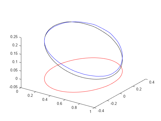
Interpolate the solution at a circle.
s = linspace(0,2*pi); x = 0.5 + 0.4*cos(s); y = 0.4*sin(s); uOut = evaluate(F,x,y);
Plot the three solution components.
npts = length(x); plot3(x,y,uOut(1:npts),"b") hold on plot3(x,y,uOut(npts+1:2*npts),"k") plot3(x,y,uOut(2*npts+1:end),"r") hold off view(35,35)
Interpolate a Time-Varying Solution
This example shows how to interpolate a solution that depends on time.
Solve the equation
on the unit disk with zero Dirichlet conditions and zero initial conditions. Solve at five times from 0 to 1.
g0 = [1;0;0;1]; % circle centered at (0,0) with radius 1 sf = 'C1'; g = decsg(g0,sf,sf'); % decomposed geometry matrix model = createpde; gm = geometryFromEdges(model,g); % Zero Dirichlet conditions applyBoundaryCondition(model,"dirichlet", ... "Edge",(1:gm.NumEdges), ... "u",0); [p,e,t] = initmesh(gm); c = 1; a = 0; f = 1; d = 1; tlist = 0:1/4:1; u = parabolic(0,tlist,model,p,e,t,c,a,f,d);
52 successful steps 0 failed attempts 106 function evaluations 1 partial derivatives 13 LU decompositions 105 solutions of linear systems
Construct an interpolant for the solution.
F = pdeInterpolant(p,t,u);
Interpolate the solution at x = 0.1
, y = -0.1
, and all available times.
x = 0.1; y = -0.1; uOut = evaluate(F,x,y)
uOut = 1×5
0 0.1809 0.2278 0.2388 0.2413
The solution starts at 0 at time 0, as it should. It grows to about 1/4 at time 1.
Interpolate to a Grid
This example shows how to interpolate an elliptic solution to a grid.
Define and Solve the Problem
Use the built-in geometry functions to create an L-shaped region with zero Dirichlet boundary conditions. Solve an elliptic PDE with coefficients , , , with zero Dirichlet boundary conditions.
[p,e,t] = initmesh("lshapeg"); % Predefined geometry u = assempde("lshapeb",p,e,t,1,0,1); % Predefined boundary condition
Create an Interpolant
Create an interpolant for the solution.
F = pdeInterpolant(p,t,u);
Create a Grid for the Solution
xgrid = -1:0.1:1; ygrid = -1:0.2:1; [X,Y] = meshgrid(xgrid,ygrid);
The resulting grid has some points that are outside the L-shaped region.
Evaluate the Solution On the Grid
uout = evaluate(F,X,Y);
The interpolated solution uout
is a column vector. You can reshape it to match the size of X
or Y
. This gives a matrix, like the output of the tri2grid
function.
Z = reshape(uout,size(X));
Input Arguments
F
— Interpolant
output of pdeInterpolant
Interpolant, specified as the output of pdeInterpolant
.
Example: F = pdeInterpolant(p,t,u)
pOut
— Query points
matrix with two or three rows
Query points, specified as a matrix with two or three rows. The first row
represents the x
component of the query points, the
second row represents the y
component, and, for 3-D
geometry, the third row represents the z
component.
evaluate
computes the interpolant at each column of
pOut
. In other words, evaluate
interpolates at the points pOut(:,k)
.
Example: pOut = [-1.5,0,1;
1,1,2.2]
Data Types: double
x
— Query point component
vector or array
Query point component, specified as a vector or array. evaluate
interpolates at either 2-D points
[x(k),y(k)]
or at 3-D points
[x(k),y(k),z(k)]
. The x
and
y
, and z
arrays must contain the
same number of entries.
evaluate
transforms query point components to the
linear index representation, such as x(:)
.
Example: x = -1:0.2:3
Data Types: double
y
— Query point component
vector or array
Query point component, specified as a vector or array. evaluate
interpolates at either 2-D points
[x(k),y(k)]
or at 3-D points
[x(k),y(k),z(k)]
. The x
and
y
, and z
arrays must contain the
same number of entries.
evaluate
transforms query point components to the
linear index representation, such as y(:)
.
Example: y = -1:0.2:3
Data Types: double
z
— Query point component
vector or array
Query point component, specified as a vector or array. evaluate
interpolates at either 2-D points
[x(k),y(k)]
or at 3-D points
[x(k),y(k),z(k)]
. The x
and
y
, and z
arrays must contain the
same number of entries.
evaluate
transforms query point components to the
linear index representation, such as z(:)
.
Example: z = -1:0.2:3
Data Types: double
Output Arguments
uOut
— Interpolated values
array
Interpolated values, returned as an array. uOut
has the
same number of columns as the data u
used in creating
F
. If u
depends on time,
uOut
contains a column for each time step. For
time-independent u
, uOut
has one
column.
The number of rows in uOut
is the number of equations
in the PDE system, N
, times the number of query points,
pOut
. The first pOut
rows
correspond to equation 1, the next pOut
rows correspond
to equation 2, and so on.
If a query point is outside the mesh, evaluate
returns NaN
for that
point.
More About
Element
An element is a basic unit in the finite-element method.
For 2-D problems, an element is a triangle in the model.Mesh.Element
property. If the triangle represents a linear element, it has nodes only at the triangle
corners. If the triangle represents a quadratic element, then it has nodes at the triangle
corners and edge centers.
For 3-D problems, an element is a tetrahedron with either four or ten points. A four-point (linear) tetrahedron has nodes only at its corners. A ten-point (quadratic) tetrahedron has nodes at its corners and at the center point of each edge.
For details, see Mesh Data.
Algorithms
For each point where a solution is requested (pOut
), there are two
steps in the interpolation process. First, the element containing
the point must be located and second, interpolation within that element must be
performed using the element shape functions and the values of the solution at the
element’s node points.
Version History
Introduced in R2014b
MATLAB Command
You clicked a link that corresponds to this MATLAB command:
Run the command by entering it in the MATLAB Command Window. Web browsers do not support MATLAB commands.
Select a Web Site
Choose a web site to get translated content where available and see local events and offers. Based on your location, we recommend that you select: .
You can also select a web site from the following list
How to Get Best Site Performance
Select the China site (in Chinese or English) for best site performance. Other MathWorks country sites are not optimized for visits from your location.
Americas
- América Latina (Español)
- Canada (English)
- United States (English)
Europe
- Belgium (English)
- Denmark (English)
- Deutschland (Deutsch)
- España (Español)
- Finland (English)
- France (Français)
- Ireland (English)
- Italia (Italiano)
- Luxembourg (English)
- Netherlands (English)
- Norway (English)
- Österreich (Deutsch)
- Portugal (English)
- Sweden (English)
- Switzerland
- United Kingdom (English)
Asia Pacific
- Australia (English)
- India (English)
- New Zealand (English)
- 中国
- 日本Japanese (日本語)
- 한국Korean (한국어)