Main Content

interpolateSolution

Interpolate PDE solution to arbitrary points

Description

uintrp = interpolateSolution(results,xq,yq) returns the interpolated values of the solution to the scalar stationary equation specified in results at the 2-D points specified in xq and yq.

example

uintrp = interpolateSolution(results,xq,yq,zq) returns the interpolated values at the 3-D points specified in xq, yq, and zq.

example

uintrp = interpolateSolution(results,querypoints) returns the interpolated values at the points in querypoints.

example

uintrp = interpolateSolution(___,iU), for any previous syntax, returns the interpolated values of the solution to the system of stationary equations for equation indices iU.

example

uintrp = interpolateSolution(___,iT) returns the interpolated values of the solution to the time-dependent or eigenvalue equation or system of such equations at times or modal indices iT. For a system of time-dependent or eigenvalue equations, specify both time/modal indices iT and equation indices iU

example

Examples

collapse all

Interpolate the solution to a scalar problem along a line and plot the result.

Create the solution to the problem -Δu=1 on the L-shaped membrane with zero Dirichlet boundary conditions.

model = createpde;
geometryFromEdges(model,@lshapeg);
applyBoundaryCondition(model,"dirichlet", ...
                             "Edge",1:model.Geometry.NumEdges, ...
                             "u",0);
specifyCoefficients(model,"m",0,...
                          "d",0,...
                          "c",1,...
                          "a",0,...
                          "f",1);
generateMesh(model,"Hmax",0.05);
results = solvepde(model);

Interpolate the solution along the straight line from (x,y) = (-1,-1) to (1,1). Plot the interpolated solution.

xq = linspace(-1,1,101);
yq = xq;

uintrp = interpolateSolution(results,xq,yq);
plot(xq,uintrp)

xlabel("x")
ylabel("u(x)")

Figure contains an axes object. The axes object with xlabel x, ylabel u(x) contains an object of type line.

Calculate the mean exit time of a Brownian particle from a region that contains absorbing (escape) boundaries and reflecting boundaries. Use the Poisson's equation with constant coefficients and 3-D rectangular block geometry to model this problem.

Create the solution for this problem.

model = createpde;
importGeometry(model,"Block.stl");
applyBoundaryCondition(model,"dirichlet","Face",[1,2,5],"u",0);
specifyCoefficients(model,"m",0,...
                          "d",0,...
                          "c",1,...
                          "a",0,...
                          "f",2);
generateMesh(model);
results = solvepde(model);

Create a grid and interpolate the solution to the grid.

[X,Y,Z] = meshgrid(0:135,0:35,0:61);
uintrp = interpolateSolution(results,X,Y,Z);
uintrp = reshape(uintrp,size(X));

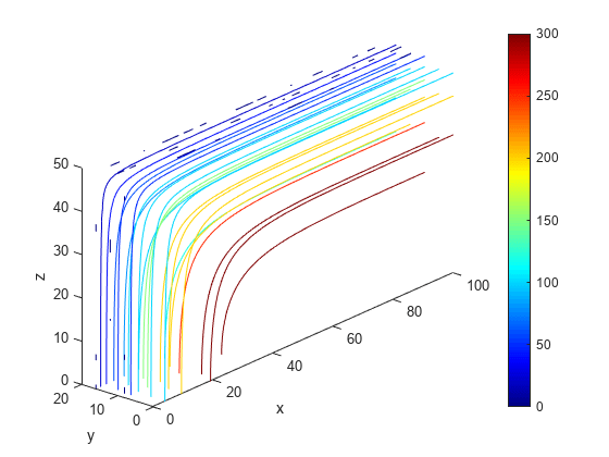
Create a contour slice plot for five fixed values of the y coordinate.

contourslice(X,Y,Z,uintrp,[],0:4:16,[])
colormap jet
xlabel("x")
ylabel("y")
zlabel("z")
xlim([0,100])
ylim([0,20])
zlim([0,50])
axis equal
view(-50,22)
colorbar

Figure contains an axes object. The axes object with xlabel x, ylabel y contains 55 objects of type patch.

Solve a scalar stationary problem and interpolate the solution to a dense grid.

Create the solution to the problem -Δu=1 on the L-shaped membrane with zero Dirichlet boundary conditions.

model = createpde;
geometryFromEdges(model,@lshapeg);
applyBoundaryCondition(model,"dirichlet", ...
                             "Edge",1:model.Geometry.NumEdges, ...
                             "u",0);
specifyCoefficients(model,"m",0,"d",0,"c",1,"a",0,"f",1);
generateMesh(model,"Hmax",0.05);
results = solvepde(model);

Interpolate the solution on the grid from –1 to 1 in each direction.

v = linspace(-1,1,101);
[X,Y] = meshgrid(v);
querypoints = [X(:),Y(:)]';
uintrp = interpolateSolution(results,querypoints);

Plot the resulting interpolation on a mesh.

uintrp = reshape(uintrp,size(X));
mesh(X,Y,uintrp)
xlabel("x")
ylabel("y")

Figure contains an axes object. The axes object with xlabel x, ylabel y contains an object of type surface.

Create the solution to a two-component system and plot the two components along a planar slice through the geometry.

Create a PDE model for two components. Import the geometry of a torus.

model = createpde(2);
importGeometry(model,"Torus.stl");
pdegplot(model,"FaceLabels","on");

Figure contains an axes object. The axes object contains 5 objects of type quiver, text, patch.

Set boundary conditions.

gfun = @(region,state)[0,region.z-40];
applyBoundaryCondition(model,"neumann","Face",1,"g",gfun);
ufun = @(region,state)[region.x-40,0];
applyBoundaryCondition(model,"dirichlet","Face",1,"u",ufun);

Set the problem coefficients.

specifyCoefficients(model,"m",0,...
                          "d",0,...
                          "c",[1;0;1;0;0;1;0;0;1;0;1;
                               0;1;0;0;1;0;1;0;0;1],...
                          "a",0,...
                          "f",[1;1]);

Create a mesh and solve the problem.

generateMesh(model);
results = solvepde(model);

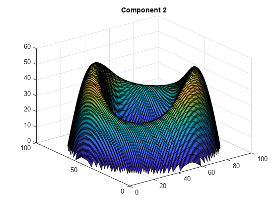
Interpolate the results on a plane that slices the torus for each of the two components.

[X,Z] = meshgrid(0:100);
Y = 15*ones(size(X));
uintrp = interpolateSolution(results,X,Y,Z,[1,2]);

Plot the two components.

sol1 = reshape(uintrp(:,1),size(X));
sol2 = reshape(uintrp(:,2),size(X));
figure
surf(X,Z,sol1)
title("Component 1")

Figure contains an axes object. The axes object with title Component 1 contains an object of type surface.

figure
surf(X,Z,sol2)
title("Component 2")

Figure contains an axes object. The axes object with title Component 2 contains an object of type surface.

Solve a scalar eigenvalue problem and interpolate one eigenvector to a grid.

Find the eigenvalues and eigenvectors for the L-shaped membrane.

model = createpde(1);
geometryFromEdges(model,@lshapeg);
applyBoundaryCondition(model,"dirichlet", ...
                             "Edge",1:model.Geometry.NumEdges, ...
                             "u",0);
specifyCoefficients(model,"m",0,...
                          "d",1,...
                          "c",1,...
                          "a",0,...
                          "f",0);
r = [0,100];
generateMesh(model,"Hmax",1/50);
results = solvepdeeig(model,r);

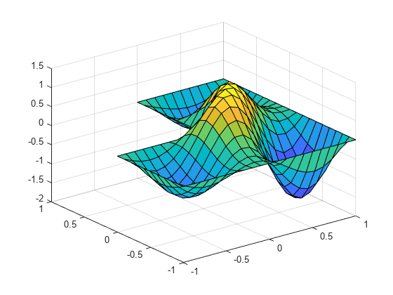
Interpolate the eigenvector corresponding to the fifth eigenvalue to a coarse grid and plot the result.

[xq,yq] = meshgrid(-1:0.1:1);
uintrp = interpolateSolution(results,xq,yq,5);
uintrp = reshape(uintrp,size(xq));
surf(xq,yq,uintrp)

Figure contains an axes object. The axes object contains an object of type surface.

Solve a system of time-dependent PDEs and interpolate the solution.

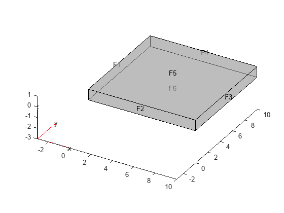
Import slab geometry for a 3-D problem with three solution components. Plot the geometry.

model = createpde(3);
importGeometry(model,"Plate10x10x1.stl");
pdegplot(model,"FaceLabels","on","FaceAlpha",0.5)

Figure contains an axes object. The axes object contains 6 objects of type quiver, text, patch, line.

Set boundary conditions such that face 2 is fixed (zero deflection in any direction) and face 5 has a load of 1e3 in the positive z-direction. This load causes the slab to bend upward. Set the initial condition that the solution is zero, and its derivative with respect to time is also zero.

applyBoundaryCondition(model,"dirichlet","Face",2,"u",[0,0,0]);
applyBoundaryCondition(model,"neumann","Face",5,"g",[0,0,1e3]);
setInitialConditions(model,0,0);

Create PDE coefficients for the equations of linear elasticity. Set the material properties to be similar to those of steel. See Linear Elasticity Equations.

E = 200e9;
nu = 0.3;
specifyCoefficients(model,"m",1,...
                          "d",0,...
                          "c",elasticityC3D(E,nu),...
                          "a",0,...
                          "f",[0;0;0]);

Generate a mesh, setting Hmax to 1.

generateMesh(model,"Hmax",1);

Solve the problem for times 0 through 5e-3 in steps of 1e-4.

tlist = 0:1e-4:5e-3;
results = solvepde(model,tlist);

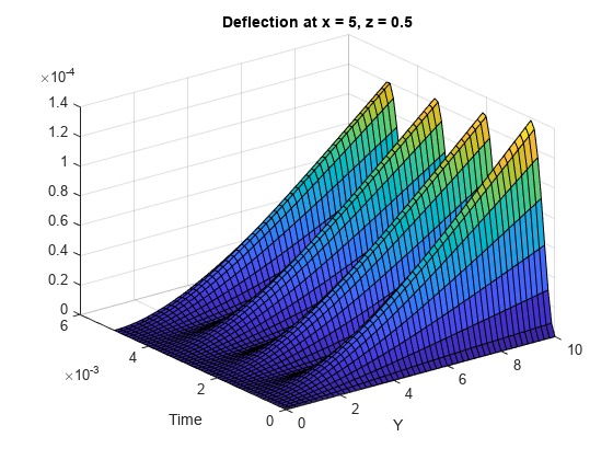
Interpolate the solution at fixed x- and z-coordinates in the centers of their ranges, 5 and 0.5 respectively. Interpolate for y from 0 through 10 in steps of 0.2. Obtain just component 3, the z-component of the solution.

yy = 0:0.2:10;
zz = 0.5*ones(size(yy));
xx = 10*zz;
component = 3;
uintrp = interpolateSolution(results,xx,yy,zz, ...
                   component,1:length(tlist));

The solution is a 51-by-1-by-51 array. Use squeeze to remove the singleton dimension. Removing the singleton dimension transforms this array to a 51-by-51 matrix which simplifies indexing into it.

uintrp = squeeze(uintrp);

Plot the solution as a function of y and time.

[X,Y] = ndgrid(yy,tlist);
figure
surf(X,Y,uintrp)
xlabel("Y")
ylabel("Time")
title("Deflection at x = 5, z = 0.5")
zlim([0,14e-5])

Figure contains an axes object. The axes object with title Deflection at x = 5, z = 0.5, xlabel Y, ylabel Time contains an object of type surface.

Input Arguments

collapse all

PDE solution, specified as a StationaryResults object, a TimeDependentResults object, or an EigenResults object. Create results using solvepde, solvepdeeig, or createPDEResults.

Example: results = solvepde(model)

x-coordinate query points, specified as a real array. interpolateSolution evaluates the solution at the 2-D coordinate points [xq(i),yq(i)] or at the 3-D coordinate points [xq(i),yq(i),zq(i)]. So xq, yq, and (if present) zq must have the same number of entries.

interpolateSolution converts query points to column vectors xq(:), yq(:), and (if present) zq(:). The returned solution is a column vector of the same size. To ensure that the dimensions of the returned solution is consistent with the dimensions of the original query points, use reshape. For example, use uintrp = reshape(gradxuintrp,size(xq)).

Data Types: double

y-coordinate query points, specified as a real array. interpolateSolution evaluates the solution at the 2-D coordinate points [xq(i),yq(i)] or at the 3-D coordinate points [xq(i),yq(i),zq(i)]. So xq, yq, and (if present) zq must have the same number of entries. Internally, interpolateSolution converts query points to the column vector yq(:).

Data Types: double

z-coordinate query points, specified as a real array. interpolateSolution evaluates the solution at the 3-D coordinate points [xq(i),yq(i),zq(i)]. So xq, yq, and zq must have the same number of entries. Internally, interpolateSolution converts query points to the column vector zq(:).

Data Types: double

Query points, specified as a real matrix with either two rows for 2-D geometry, or three rows for 3-D geometry. interpolateSolution evaluates the solution at the coordinate points querypoints(:,i), so each column of querypoints contains exactly one 2-D or 3-D query point.

Example: For 2-D geometry, querypoints = [0.5,0.5,0.75,0.75; 1,2,0,0.5]

Data Types: double

Equation indices, specified as a vector of positive integers. Each entry in iU specifies an equation index.

Example: iU = [1,5] specifies the indices for the first and fifth equations.

Data Types: double

Time or mode indices, specified as a vector of positive integers. Each entry in iT specifies a time index for time-dependent solutions, or a mode index for eigenvalue solutions.

Example: iT = 1:5:21 specifies the time or mode for every fifth solution up to 21.

Data Types: double

Output Arguments

collapse all

Solution at query points, returned as an array. For query points that are outside the geometry, uintrp = NaN. For details about dimensions of the solution, see Dimensions of Solutions, Gradients, and Fluxes.

Version History

Introduced in R2015b