Main Content

StationaryResults

Time-independent PDE solution and derived quantities

Description

A StationaryResults object contains the solution of a PDE and its gradients in a form convenient for plotting and postprocessing.

  • A StationaryResults object contains the solution and its gradient calculated at the nodes of the triangular or tetrahedral mesh, generated by generateMesh.

  • Solution values at the nodes appear in the NodalSolution property.

  • The three components of the gradient of the solution values at the nodes appear in the XGradients, YGradients, and ZGradients properties.

  • The array dimensions of NodalSolution, XGradients, YGradients, and ZGradients enable you to extract solution and gradient values for specified equation indices in a PDE system.

To interpolate the solution or its gradient to a custom grid (for example, specified by meshgrid), use interpolateSolution or evaluateGradient.

Creation

There are several ways to create a StationaryResults object:

  • Solve a time-independent problem using the solvepde function. This function returns a PDE solution as a StationaryResults object. This is the recommended approach.

  • Solve a time-independent problem using the assempde or pdenonlin function. Then use the createPDEResults function to obtain a StationaryResults object from a PDE solution returned by assempde or pdenonlin. Note that assempde and pdenonlin are legacy functions. They are not recommended for solving PDE problems.

Properties

expand all

This property is read-only.

Finite element mesh, returned as a FEMesh object.

This property is read-only.

Solution values at the nodes, returned as a vector or array. For details about the dimensions of NodalSolution, see Dimensions of Solutions, Gradients, and Fluxes.

Data Types: double

This property is read-only.

x-component of the gradient at the nodes, returned as a vector or array. For details about the dimensions of XGradients, see Dimensions of Solutions, Gradients, and Fluxes.

Data Types: double

This property is read-only.

y-component of the gradient at the nodes, returned as a vector or array. For details about the dimensions of YGradients, see Dimensions of Solutions, Gradients, and Fluxes.

Data Types: double

This property is read-only.

z-component of the gradient at the nodes, returned as a vector or array. For details about the dimensions of ZGradients, see Dimensions of Solutions, Gradients, and Fluxes.

Data Types: double

Object Functions

evaluateCGradientEvaluate flux of PDE solution
evaluateGradientEvaluate gradients of PDE solutions at arbitrary points
interpolateSolutionInterpolate PDE solution to arbitrary points

Examples

collapse all

Create a PDE model for a system of three equations. Import the geometry of a bracket and plot the face labels.

model = createpde(3);
importGeometry(model,"BracketWithHole.stl");

figure
pdegplot(model,"FaceLabels","on")
view(30,30)
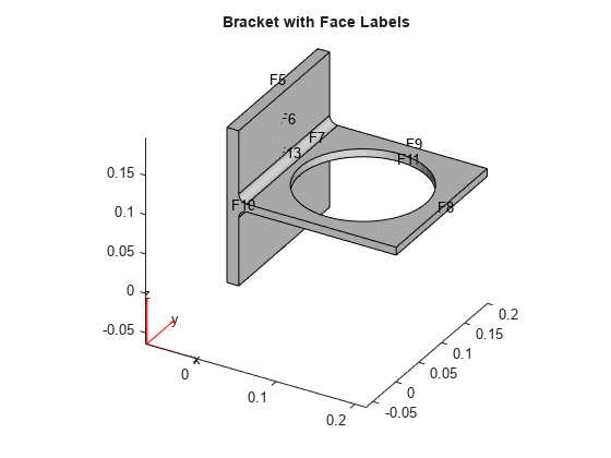
title("Bracket with Face Labels")

Figure contains an axes object. The axes object with title Bracket with Face Labels contains 6 objects of type quiver, text, patch, line.

figure
pdegplot(model,"FaceLabels","on")
view(-134,-32)
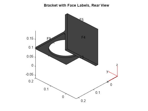
title("Bracket with Face Labels, Rear View")

Figure contains an axes object. The axes object with title Bracket with Face Labels, Rear View contains 6 objects of type quiver, text, patch, line.

Set boundary conditions such that face 4 is immobile, and face 8 has a force in the negative z direction.

applyBoundaryCondition(model,"dirichlet","Face",4,"u",[0,0,0]);
applyBoundaryCondition(model,"neumann","Face",8,"g",[0,0,-1e4]);

Set coefficients that represent the equations of linear elasticity. See Linear Elasticity Equations.

E = 200e9;
nu = 0.3;
specifyCoefficients(model,"m",0,...
                          "d",0,...
                          "c",elasticityC3D(E,nu),...
                          "a",0,...
                          "f",[0;0;0]);

Create a mesh.

generateMesh(model,"Hmax",1e-2);

Solve the PDE.

results = solvepde(model)
results = 
  StationaryResults with properties:

    NodalSolution: [14093x3 double]
       XGradients: [14093x3 double]
       YGradients: [14093x3 double]
       ZGradients: [14093x3 double]
             Mesh: [1x1 FEMesh]

Access the solution at the nodal locations.

u = results.NodalSolution;

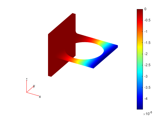
Plot the solution for the z-component, which is component 3.

pdeplot3D(model,"ColorMapData",u(:,3))

Figure contains an axes object. The hidden axes object contains 5 objects of type patch, quiver, text.

Obtain a StationaryResults object from a legacy solver together with createPDEResults.

Create a PDE model for a system of three equations. Import the geometry of a bracket and plot the face labels.

model = createpde(3);
importGeometry(model,"BracketWithHole.stl");

figure
pdegplot(model,"FaceLabels","on")
view(30,30)
title("Bracket with Face Labels")

Figure contains an axes object. The axes object with title Bracket with Face Labels contains 6 objects of type quiver, text, patch, line.

figure
pdegplot(model,"FaceLabels","on")
view(-134,-32)
title("Bracket with Face Labels, Rear View")

Figure contains an axes object. The axes object with title Bracket with Face Labels, Rear View contains 6 objects of type quiver, text, patch, line.

Set boundary conditions such that F4 is immobile, and F8 has a force in the negative z direction.

applyBoundaryCondition(model,"dirichlet","Face",4,"u",[0,0,0]);
applyBoundaryCondition(model,"neumann","Face",8,"g",[0,0,-1e4]);

Set coefficients for a legacy solver that represent the equations of linear elasticity. See Linear Elasticity Equations.

E = 200e9;
nu = 0.3;
c = elasticityC3D(E,nu);
a = 0;
f = [0;0;0];

Create a mesh.

generateMesh(model,"Hmax",1e-2);

Solve the problem using a legacy solver.

u = assempde(model,c,a,f);

Create a StationaryResults object from the solution.

results = createPDEResults(model,u)
results = 
  StationaryResults with properties:

    NodalSolution: [14093x3 double]
       XGradients: [14093x3 double]
       YGradients: [14093x3 double]
       ZGradients: [14093x3 double]
             Mesh: [1x1 FEMesh]

Access the solution at the nodal locations.

u = results.NodalSolution;

Plot the solution for the z-component, which is component 3.

pdeplot3D(model,"ColorMapData",u(:,3))

Figure contains an axes object. The hidden axes object contains 5 objects of type patch, quiver, text.

Version History

Introduced in R2016a

expand all