Main Content

createPDEResults

Create solution object

This page describes the legacy workflow. New features might not be compatible with the legacy workflow. For the corresponding step in the recommended workflow, see solvepde and solvepdeeig.

The original (R2015b) version of createPDEResults had only one syntax, and created a PDEResults object. Beginning with R2016a, you generally do not need to use createPDEResults, because the solvepde and solvepdeeig functions return solution objects. Furthermore, createPDEResults returns an object of a newer type than PDEResults. If you open an existing PDEResults object, it is converted to a StationaryResults object.

If you use one of the older solvers such as adaptmesh, then you can use createPDEResults to obtain a solution object. Stationary and time-dependent solution objects have gradients available, whereas PDEResults did not include gradients.

Description

results = createPDEResults(model,u) creates a StationaryResults solution object from model and its solution u.

This syntax is equivalent to results = createPDEResults(model,u,"stationary").

example

results = createPDEResults(model,u,utimes,"time-dependent") creates a TimeDependentResults solution object from model, its solution u, and the times utimes.

example

results = createPDEResults(model,eigenvectors,eigenvalues,"eigen") creates an EigenResults solution object from model, its eigenvector solution eigenvectors, and its eigenvalues eigenvalues.

example

Examples

collapse all

Create a StationaryResults object from the solution to an elliptic system.

Create a PDE model for a system of three equations. Import the geometry of a bracket and plot the face labels.

model = createpde(3);
importGeometry(model,"BracketWithHole.stl");
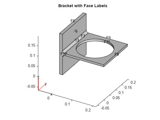
figure
pdegplot(model,"FaceLabels","on")
view(30,30)
title("Bracket with Face Labels")

Figure contains an axes object. The axes object with title Bracket with Face Labels contains 6 objects of type quiver, text, patch, line.

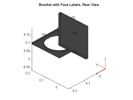
figure
pdegplot(model,"FaceLabels","on")
view(-134,-32)
title("Bracket with Face Labels, Rear View")

Figure contains an axes object. The axes object with title Bracket with Face Labels, Rear View contains 6 objects of type quiver, text, patch, line.

Set boundary conditions: face 3 is immobile, and there is a force in the negative z direction on face 6.

applyBoundaryCondition(model,"dirichlet","Face",4,"u",[0,0,0]);
applyBoundaryCondition(model,"neumann","Face",8,"g",[0,0,-1e4]);

Set coefficients that represent the equations of linear elasticity.

E = 200e9;
nu = 0.3;
c = elasticityC3D(E,nu);
a = 0;
f = [0;0;0];

Create a mesh and solve the problem.

generateMesh(model,"Hmax",1e-2);
u = assempde(model,c,a,f);

Create a StationaryResults object from the solution.

results = createPDEResults(model,u)
results = 
  StationaryResults with properties:

    NodalSolution: [14093x3 double]
       XGradients: [14093x3 double]
       YGradients: [14093x3 double]
       ZGradients: [14093x3 double]
             Mesh: [1x1 FEMesh]

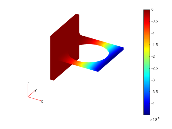
Plot the solution for the z-component, which is component 3.

pdeplot3D(model,"ColorMapData",results.NodalSolution(:,3))

Figure contains an axes object. The hidden axes object contains 5 objects of type patch, quiver, text.

Obtain a solution from a parabolic problem.

The problem models heat flow in a solid.

model = createpde();
importGeometry(model,"Tetrahedron.stl");
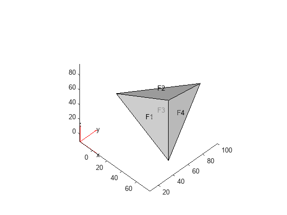
pdegplot(model,"FaceLabels","on","FaceAlpha",0.5)
view(45,45)

Figure contains an axes object. The axes object contains 6 objects of type quiver, text, patch, line.

Set the temperature on face 2 to 100. Leave the other boundary conditions at their default values (insulating).

applyBoundaryCondition(model,"dirichlet","Face",2,"u",100);

Set the coefficients to model a parabolic problem with 0 initial temperature.

d = 1;
c = 1;
a = 0;
f = 0;
u0 = 0;

Create a mesh and solve the PDE for times from 0 through 200 in steps of 10.

tlist = 0:10:200;
generateMesh(model);
u = parabolic(u0,tlist,model,c,a,f,d);
171 successful steps
0 failed attempts
326 function evaluations
1 partial derivatives
29 LU decompositions
325 solutions of linear systems

Create a TimeDependentResults object from the solution.

results = createPDEResults(model,u,tlist,"time-dependent");

Plot the solution on the surface of the geometry at time 100.

pdeplot3D(model,"ColorMapData",results.NodalSolution(:,11))

Figure contains an axes object. The hidden axes object contains 5 objects of type patch, quiver, text.

Create an EigenResults object from the solution to an eigenvalue problem.

Create the geometry and mesh for the L-shaped membrane. Apply Dirichlet boundary conditions to all edges.

model = createpde;
geometryFromEdges(model,@lshapeg);
generateMesh(model,"Hmax",0.05,"GeometricOrder","linear");
applyBoundaryCondition(model,"dirichlet", ...
                             "Edge",1:model.Geometry.NumEdges, ...
                             "u",0);

Solve the eigenvalue problem for coefficients c = 1, a = 0, and d = 1. Obtain solutions for eigenvalues from 0 through 100.

c = 1;
a = 0;
d = 1;
r = [0,100];
[eigenvectors,eigenvalues] = pdeeig(model,c,a,d,r);

Create an EigenResults object from the solution.

results = createPDEResults(model,eigenvectors,eigenvalues,"eigen")
results = 
  EigenResults with properties:

    Eigenvectors: [1458x12 double]
     Eigenvalues: [12x1 double]
            Mesh: [1x1 FEMesh]

Plot the solution for mode 10.

pdeplot(model,"XYData",results.Eigenvectors(:,10))

Figure contains an axes object. The axes object contains an object of type patch.

Input Arguments

collapse all

PDE model, specified as a PDEModel object.

Example: model = createpde

PDE solution, specified as a vector or matrix.

Example: u = assempde(model,c,a,f);

Times for a PDE solution, specified as a monotone vector. These times should be the same as the tlist times that you specified for the solution by the hyperbolic or parabolic solvers.

Example: utimes = 0:0.2:5;

Eigenvector solution, specified as a matrix. Suppose

  • Np is the number of mesh nodes

  • N is the number of equations

  • ev is the number of eigenvalues specified in eigenvalues

Then eigenvectors has size Np-by-N-by-ev. Each column of eigenvectors corresponds to the eigenvectors of one eigenvalue. In each column, the first Np elements correspond to the eigenvector of equation 1 evaluated at the mesh nodes, the next Np elements correspond to equation 2, and so on.

Eigenvalue solution, specified as a vector.

Output Arguments

collapse all

PDE solution, specified as a StationaryResults object, a TimeDependentResults object, or an EigenResults object. Create results using solvepde, solvepdeeig, or createPDEResults.

Example: results = solvepde(model)

Tips

Algorithms

The procedure for evaluating gradients at nodal locations is as follows:

  1. Calculate the gradients at the Gauss points located inside each element.

  2. Extrapolate the gradients at the nodal locations.

  3. Average the value of the gradient from all elements that meet at the nodal point. This step is needed because of the inter-element discontinuity of gradients. The elements that connect at the same nodal point give different extrapolated values of the gradient for the point. createPDEResults performs area-weighted averaging for 2-D meshes and volume-weighted averaging for 3-D meshes.
    Four mesh elements meeting at one node contribute to the averaged value of the gradient at the node

Version History

Introduced in R2015b

expand all