evaluateGradient

Evaluate gradients of PDE solutions at arbitrary points

Syntax

[gradx,grady]
= evaluateGradient(results,xq,yq)

[gradx,grady,gradz]
= evaluateGradient(results,xq,yq,zq)

[___] = evaluateGradient(results,querypoints)

[___] = evaluateGradient(___,iU)

[___] = evaluateGradient(___,iT)

Description

[gradx,grady] = evaluateGradient(results,xq,yq) returns the interpolated values of gradients of the PDE solution results at the 2-D points specified in xq and yq.

example

[gradx,grady,gradz] = evaluateGradient(results,xq,yq,zq) returns the interpolated gradients at the 3-D points specified in xq, yq, and zq.

example

[___] = evaluateGradient(results,querypoints) returns the interpolated values of the gradients at the points specified in querypoints.

example

[___] = evaluateGradient(___,iU) returns the interpolated values of the gradients for the system of equations for equation indices (components) iU. When solving a system of elliptic PDEs, specify iU after the input arguments in any of the previous syntaxes.

The first dimension of gradx, grady, and, in 3-D case, gradz corresponds to query points. The second dimension corresponds to equation indices iU.

example

[___] = evaluateGradient(___,iT) returns the interpolated values of the gradients for the time-dependent equation or system of time-dependent equations at times iT. When evaluating gradient for a time-dependent PDE, specify iT after the input arguments in any of the previous syntaxes. For a system of time-dependent equations, specify both time indices iT and equation indices (components) iU.

The first dimension of gradx, grady, and, in 3-D case, gradz corresponds to query points. For a single time-dependent PDE, the second dimension corresponds to time-steps iT. For a system of time-dependent PDEs, the second dimension corresponds to equation indices iU, and the third dimension corresponds to time-steps iT.

example

Examples

collapse all

Evaluate Gradients for Scalar Elliptic Problem

Open Live Script

Evaluate gradients of the solution to a scalar elliptic problem along a line. Plot the results.

Create the solution to the problem $- Δ u = 1$ on the L-shaped membrane with zero Dirichlet boundary conditions.

model = createpde;
geometryFromEdges(model,@lshapeg);
applyBoundaryCondition(model,"dirichlet", ...
                             "Edge",1:model.Geometry.NumEdges, ...
                             "u",0);
specifyCoefficients(model,"m",0,...
                          "d",0,...
                          "c",1,...
                          "a",0,...
                          "f",1);
generateMesh(model,"Hmax",0.05);
results = solvepde(model);

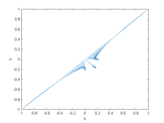
Evaluate gradients of the solution along the straight line from (x,y)=(-1,-1) to (1,1). Plot the results as a quiver plot by using quiver.

xq = linspace(-1,1,101);
yq = xq;
[gradx,grady] = evaluateGradient(results,xq,yq);

gradx = reshape(gradx,size(xq));
grady = reshape(grady,size(yq));

quiver(xq,yq,gradx,grady)
xlabel("x")
ylabel("y")

Figure contains an axes object. The axes object with xlabel x, ylabel y contains an object of type quiver.

Evaluate Gradients for Poisson's Equation

Open Live Script

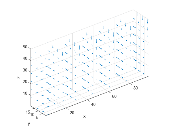
Calculate gradients for the mean exit time of a Brownian particle from a region that contains absorbing (escape) boundaries and reflecting boundaries. Use the Poisson's equation with constant coefficients and 3-D rectangular block geometry to model this problem.

Create the solution for this problem.

model = createpde;
importGeometry(model,"Block.stl");
applyBoundaryCondition(model,"dirichlet", ...
                             "Face",[1,2,5], ...
                             "u",0);
specifyCoefficients(model,"m",0,...
                          "d",0,...
                          "c",1,...
                          "a",0,...
                          "f",2);
generateMesh(model);
results = solvepde(model);

Create a grid and interpolate gradients of the solution to the grid.

[X,Y,Z] = meshgrid(1:16:100,1:6:20,1:7:50);
[gradx,grady,gradz] = evaluateGradient(results,X,Y,Z);

Reshape the gradients to the shape of the grid and plot the gradients.

gradx = reshape(gradx,size(X));
grady = reshape(grady,size(Y));
gradz = reshape(gradz,size(Z));

quiver3(X,Y,Z,gradx,grady,gradz)
axis equal
xlabel("x")
ylabel("y")
zlabel("z")

Figure contains an axes object. The axes object with xlabel x, ylabel y contains an object of type quiver.

Evaluate Gradients Using Query Matrix

Open Live Script

Solve a scalar elliptic problem and interpolate gradients of the solution to a dense grid. Use a query matrix to specify the grid.

Create the solution to the problem $- Δ u = 1$ on the L-shaped membrane with zero Dirichlet boundary conditions.

model = createpde;
geometryFromEdges(model,@lshapeg);
applyBoundaryCondition(model,"dirichlet", ...
                             "Edge",1:model.Geometry.NumEdges, ...
                             "u",0);
specifyCoefficients(model,"m",0,...
                          "d",0,...
                          "c",1,...
                          "a",0,...
                          "f",1);
generateMesh(model,"Hmax",0.05);
results = solvepde(model);

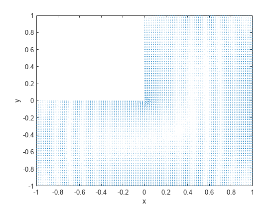
Interpolate gradients of the solution to the grid from -1 to 1 in each direction. Plot the result using the quiver plotting function.

v = linspace(-1,1,101);
[X,Y] = meshgrid(v);
querypoints = [X(:),Y(:)]';

[gradx,grady] = evaluateGradient(results,querypoints);
quiver(X(:),Y(:),gradx,grady)
xlabel("x")
ylabel("y")

Figure contains an axes object. The axes object with xlabel x, ylabel y contains an object of type quiver.

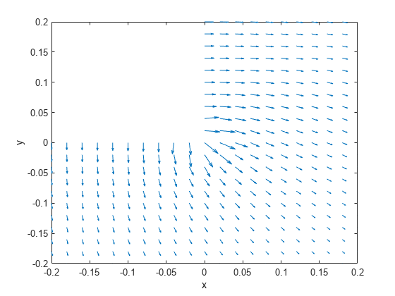
Zoom in on a particular part of the plot to see more details. For example, limit the plotting range to 0.2 in each direction.

axis([-0.2 0.2 -0.2 0.2])

Figure contains an axes object. The axes object with xlabel x, ylabel y contains an object of type quiver.

Evaluate Gradients of Solution of Elliptic System

Open Live Script

Evaluate gradients of the solution to a two-component elliptic system and plot the results.

Create a PDE model for two components.

model = createpde(2);

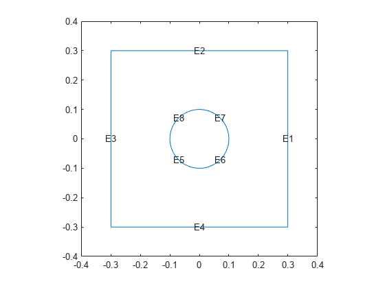
Create the 2-D geometry as a rectangle with a circular hole in its center. For details about creating the geometry, see the example in Solve PDEs with Constant Boundary Conditions.

R1 = [3,4,-0.3,0.3,0.3,-0.3,-0.3,-0.3,0.3,0.3]';
C1 = [1,0,0,0.1]';
C1 = [C1;zeros(length(R1)-length(C1),1)];
geom = [R1,C1];
ns = (char('R1','C1'))';
sf = 'R1 - C1';
g = decsg(geom,sf,ns);

Include the geometry in the model and view the geometry.

geometryFromEdges(model,g);
pdegplot(model,"EdgeLabels","on")
axis equal
axis([-0.4,0.4,-0.4,0.4])

Figure contains an axes object. The axes object contains 9 objects of type line, text.

Set the boundary conditions and coefficients.

specifyCoefficients(model,"m",0,...
                          "d",0,...
                          "c",1,...
                          "a",0,...
                          "f",[2; -2]);

applyBoundaryCondition(model,"dirichlet", ...
                             "Edge",3,"u",[-1,1]);
applyBoundaryCondition(model,"dirichlet", ...
                             "Edge",1,"u",[1,-1]);
applyBoundaryCondition(model,"neumann", ...
                             "Edge",[2,4:8],"g",[0,0]);

Create a mesh and solve the problem.

generateMesh(model,"Hmax",0.1);
results = solvepde(model);

Interpolate the gradients of the solution to the grid from -0.3 to 0.3 in each direction for each of the two components.

v = linspace(-0.3,0.3,15);
[X,Y] = meshgrid(v);

[gradx,grady] = evaluateGradient(results,X,Y,[1,2]);

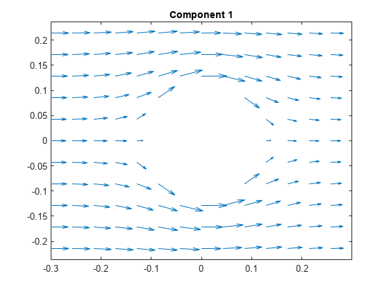
Plot the gradients for the first component.

figure
gradx1 = gradx(:,1);
grady1 = grady(:,1);
quiver(X(:),Y(:),gradx1,grady1)
title("Component 1")
axis equal
xlim([-0.3,0.3])

Figure contains an axes object. The axes object with title Component 1 contains an object of type quiver.

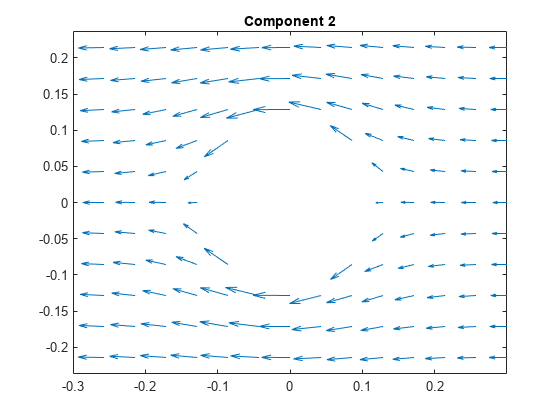
Plot the gradients for the second component.

figure
gradx2 = gradx(:,2);
grady2 = grady(:,2);
quiver(X(:),Y(:),gradx2,grady2)
title("Component 2")
axis equal
xlim([-0.3,0.3])

Figure contains an axes object. The axes object with title Component 2 contains an object of type quiver.

Evaluate Gradients of Solution of Hyperbolic System

Open Live Script

Solve a system of hyperbolic PDEs and evaluate gradients.

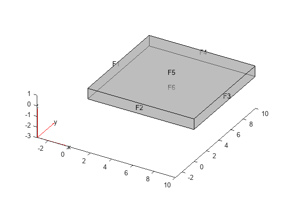
Import slab geometry for a 3-D problem with three solution components. Plot the geometry.

model = createpde(3);
importGeometry(model,"Plate10x10x1.stl");
pdegplot(model,"FaceLabels","on","FaceAlpha",0.5)

Figure contains an axes object. The axes object contains 6 objects of type quiver, text, patch, line.

Set boundary conditions such that face 2 is fixed (zero deflection in any direction) and face 5 has a load of 1e3 in the positive z-direction. This load causes the slab to bend upward. Set the initial condition that the solution is zero, and its derivative with respect to time is also zero.

applyBoundaryCondition(model,"dirichlet","Face",2,"u",[0,0,0]);
applyBoundaryCondition(model,"neumann","Face",5,"g",[0,0,1e3]);
setInitialConditions(model,0,0);

Create PDE coefficients for the equations of linear elasticity. Set the material properties to be similar to those of steel. See Linear Elasticity Equations.

E = 200e9;
nu = 0.3;
specifyCoefficients(model,"m",1,...
                          "d",0,...
                          "c",elasticityC3D(E,nu),...
                          "a",0,...
                          "f",[0;0;0]);

Generate a mesh, setting Hmax to 1.

generateMesh(model,"Hmax",1);

Solve the problem for times 0 through 5e-3 in steps of 1e-4. You might have to wait a few minutes for the solution.

tlist = 0:5e-4:5e-3;
results = solvepde(model,tlist);

Evaluate the gradients of the solution at fixed x- and z-coordinates in the centers of their ranges, 5 and 0.5 respectively. Evaluate for y from 0 through 10 in steps of 0.2. Obtain just component 3, the z-component.

yy = 0:0.2:10;
zz = 0.5*ones(size(yy));
xx = 10*zz;
component = 3;
[gradx,grady,gradz] = evaluateGradient(results,xx,yy,zz, ...
                                 component,1:length(tlist));

The three projections of the gradients of the solution are 51-by-1-by-51 arrays. Use squeeze to remove the singleton dimension. Removing the singleton dimension transforms these arrays to 51-by-51 matrices which simplifies indexing into them.

gradx = squeeze(gradx);
grady = squeeze(grady);
gradz = squeeze(gradz);

Plot the interpolated gradient component grady along the y axis for the following six values from the time interval tlist.

figure
t = [1:2:11];
for i = t
  p(i) = plot(yy,grady(:,i),"DisplayName", ...
              strcat("t=",num2str(tlist(i))));
  hold on
end
legend(p(t))
xlabel("y")
ylabel("grady")
ylim([-5e-6, 20e-6])

Figure contains an axes object. The axes object with xlabel y, ylabel grady contains 6 objects of type line. These objects represent t=0, t=0.001, t=0.002, t=0.003, t=0.004, t=0.005.

Input Arguments

collapse all

`results` — PDE solution
`StationaryResults` object | `TimeDependentResults` object

PDE solution, specified as a StationaryResults object or a TimeDependentResults object. Create results using solvepde or createPDEResults.

Example: results = solvepde(model)

`xq` — x-coordinate query points
real array

x-coordinate query points, specified as a real array. evaluateGradient evaluates the gradients of the solution at the 2-D coordinate points [xq(i),yq(i)] or at the 3-D coordinate points [xq(i),yq(i),zq(i)]. So xq, yq, and (if present) zq must have the same number of entries.

evaluateGradient converts query points to column vectors xq(:), yq(:), and (if present) zq(:). For a single stationary PDE, the result consists of column vectors of the same size. To ensure that the dimensions of the gradient components are consistent with the dimensions of the original query points, use reshape. For example, use gradx = reshape(gradx,size(xq)).

For a time-dependent PDE or a system of PDEs, the first dimension of the resulting arrays corresponds to spatial points specified by the column vectors xq(:), yq(:), and (if present) zq(:).

Data Types: double

`yq` — y-coordinate query points
real array

y-coordinate query points, specified as a real array. evaluateGradient evaluates the gradients of the solution at the 2-D coordinate points [xq(i),yq(i)] or at the 3-D coordinate points [xq(i),yq(i),zq(i)]. So xq, yq, and (if present) zq must have the same number of entries.

For a time-dependent PDE or a system of PDEs, the first dimension of the resulting arrays corresponds to spatial points specified by the column vectors xq(:), yq(:), and (if present) zq(:).

Data Types: double

`zq` — z-coordinate query points
real array

z-coordinate query points, specified as a real array. evaluateGradient evaluates the gradients of the solution at the 3-D coordinate points [xq(i),yq(i),zq(i)]. So xq, yq, and zq must have the same number of entries.

For a time-dependent PDE or a system of PDEs, the first dimension of the resulting arrays corresponds to spatial points specified by the column vectors xq(:), yq(:), and (if present) zq(:).

Data Types: double

`querypoints` — Query points
real matrix

Query points, specified as a real matrix with either two rows for 2-D geometry, or three rows for 3-D geometry. evaluateGradient evaluates the gradients of the solution at the coordinate points querypoints(:,i), so each column of querypoints contains exactly one 2-D or 3-D query point.

Example: For 2-D geometry, querypoints = [0.5,0.5,0.75,0.75; 1,2,0,0.5]

Data Types: double

`iU` — Equation indices
vector of positive integers

Equation indices, specified as a vector of positive integers. Each entry in iU specifies an equation index.

Example: iU = [1,5] specifies the indices for the first and fifth equations.

Data Types: double

`iT` — Time indices
vector of positive integers

Time indices, specified as a vector of positive integers. Each entry in iT specifies a time index.

Example: iT = 1:5:21 specifies every fifth time-step up to 21.

Data Types: double

Output Arguments

collapse all

`gradx` — x-component of the gradient
array

x-component of the gradient, returned as an array. For query points that are outside the geometry, gradx = NaN. For information about the size of gradx, see Dimensions of Solutions, Gradients, and Fluxes.

`grady` — y-component of the gradient
array

y-component of the gradient, returned as an array. For query points that are outside the geometry, grady = NaN. For information about the size of grady, see Dimensions of Solutions, Gradients, and Fluxes.

`gradz` — z-component of the gradient
array

z-component of the gradient, returned as an array. For query points that are outside the geometry, gradz = NaN. For information about the size of gradz, see Dimensions of Solutions, Gradients, and Fluxes.

Tips

The results object contains the solution and its gradient calculated at the nodal points of the triangular or tetrahedral mesh. You can access the solution and three components of the gradient at nodal points by using dot notation.

interpolateSolution and evaluateGradient let you interpolate the solution and its gradient to a custom grid, for example, specified by meshgrid.

Version History

Introduced in R2016a

evaluateGradient

Syntax

Description

Examples

Evaluate Gradients for Scalar Elliptic Problem

Evaluate Gradients for Poisson's Equation

Evaluate Gradients Using Query Matrix

Evaluate Gradients of Solution of Elliptic System

Evaluate Gradients of Solution of Hyperbolic System

Input Arguments

`results` — PDE solution
`StationaryResults` object | `TimeDependentResults` object

`xq` — x-coordinate query points
real array

`yq` — y-coordinate query points
real array

`zq` — z-coordinate query points
real array

`querypoints` — Query points
real matrix

`iU` — Equation indices
vector of positive integers

`iT` — Time indices
vector of positive integers

Output Arguments

`gradx` — x-component of the gradient
array

`grady` — y-component of the gradient
array

`gradz` — z-component of the gradient
array

Tips

Version History

See Also

Topics

evaluateGradient

Syntax

Description

Examples

Evaluate Gradients for Scalar Elliptic Problem

Evaluate Gradients for Poisson's Equation

Evaluate Gradients Using Query Matrix

Evaluate Gradients of Solution of Elliptic System

Evaluate Gradients of Solution of Hyperbolic System

Input Arguments

results — PDE solution StationaryResults object | TimeDependentResults object

xq — x-coordinate query points real array

yq — y-coordinate query points real array

zq — z-coordinate query points real array

querypoints — Query points real matrix

iU — Equation indices vector of positive integers

iT — Time indices vector of positive integers

Output Arguments

gradx — x-component of the gradient array

grady — y-component of the gradient array

gradz — z-component of the gradient array

Tips

Version History

See Also

Topics

`results` — PDE solution
`StationaryResults` object | `TimeDependentResults` object

`xq` — x-coordinate query points
real array

`yq` — y-coordinate query points
real array

`zq` — z-coordinate query points
real array

`querypoints` — Query points
real matrix

`iU` — Equation indices
vector of positive integers

`iT` — Time indices
vector of positive integers

`gradx` — x-component of the gradient
array

`grady` — y-component of the gradient
array

`gradz` — z-component of the gradient
array