interpolateStrain
Interpolate strain at arbitrary spatial locations
Syntax
Description
intrpStrain = interpolateStrain(structuralresults,xq,yq)xq and yq. For transient and
frequency-response structural problems, interpolateStrain
interpolates strain for all time or frequency steps, respectively.
intrpStrain = interpolateStrain(structuralresults,xq,yq,zq)xq, yq, and
zq.
intrpStrain = interpolateStrain(structuralresults,querypoints)querypoints.
Examples
Create an femodel object for static structural analysis and include a unit square geometry into the model.
model = femodel(AnalysisType="structuralStatic", ...
                Geometry=@squareg);
Plot the geometry.
pdegplot(model.Geometry,EdgeLabels="on")
xlim([-1.1 1.1])
ylim([-1.1 1.1])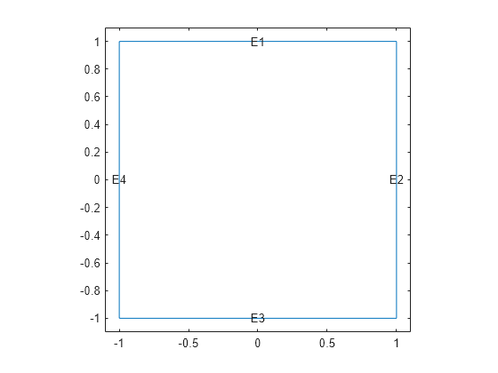
Switch the problem type to plane-strain.
model.PlanarType = "planeStrain";Specify Young's modulus and Poisson's ratio.
model.MaterialProperties = ...
    materialProperties(YoungsModulus=210E3, ...
                       PoissonsRatio=0.3);
Specify the x-component of the enforced displacement for edge 1.
model.EdgeBC(1) = edgeBC(XDisplacement=0.001);
Specify that edge 3 is a fixed boundary.
model.EdgeBC(3) = edgeBC(Constraint="fixed");Generate a mesh and solve the problem.
model = generateMesh(model);
R = solve(model);
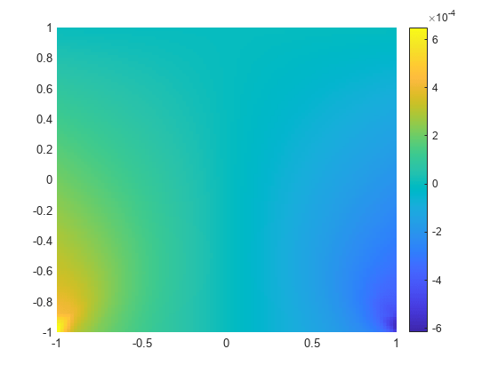
Create a grid and interpolate the x- and y-components of the normal strain to the grid.
v = linspace(-1,1,101);
[X,Y] = meshgrid(v);
intrpStrain = interpolateStrain(R,X,Y);
Reshape the x-component of the normal strain to the shape of the grid and plot it.
exx = reshape(intrpStrain.exx,size(X));
px = pcolor(X,Y,exx);
px.EdgeColor="none";
colorbar
axis equal

Reshape the y-component of the normal strain to the shape of the grid and plot it.
eyy = reshape(intrpStrain.eyy,size(Y));
figure
py = pcolor(X,Y,eyy);
py.EdgeColor="none";
colorbar
axis equal
Analyze a bimetallic cable under tension, and interpolate strain on a cross-section of the cable.
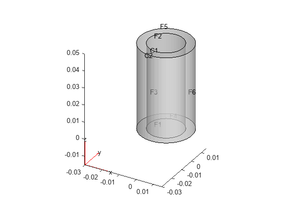
Create and plot a geometry representing a bimetallic cable.
gm = multicylinder([0.01,0.015],0.05);
pdegplot(gm,FaceLabels="on", ...
            CellLabels="on", ...
            FaceAlpha=0.5)
Create an femodel for static structural analysis and include the geometry into the model.
model = femodel(AnalysisType="structuralStatic", ...
                Geometry=gm);
Specify Young's modulus and Poisson's ratio for each metal.
model.MaterialProperties(1) = ...
    materialProperties(YoungsModulus=110E9, ...
                       PoissonsRatio=0.28);
model.MaterialProperties(2) = ...
    materialProperties(YoungsModulus=210E9, ...
                       PoissonsRatio=0.3);
Specify that faces 1 and 4 are fixed boundaries.
model.FaceBC([1 4]) = faceBC(Constraint="fixed");Specify the surface traction for faces 2 and 5.
model.FaceLoad([2 5]) = faceLoad(SurfaceTraction=[0;0;100]);
Generate a mesh and solve the problem.
model = generateMesh(model);
R = solve(model)
R =
  StaticStructuralResults with properties:

      Displacement: [1×1 FEStruct]
            Strain: [1×1 FEStruct]
            Stress: [1×1 FEStruct]
    VonMisesStress: [23098×1 double]
              Mesh: [1×1 FEMesh]
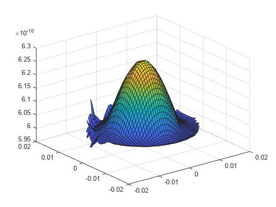
Define the coordinates of a midspan cross-section of the cable.
[X,Y] = meshgrid(linspace(-0.015,0.015,50));
Z = ones(size(X))*0.025;
Interpolate the strain and plot the result.
intrpStrain = interpolateStrain(R,X,Y,Z);
surf(X,Y,reshape(intrpStrain.ezz,size(X)))
Alternatively, you can specify the grid by using a matrix of query points.
querypoints = [X(:),Y(:),Z(:)]';
intrpStrain = interpolateStrain(R,querypoints);
surf(X,Y,reshape(intrpStrain.ezz,size(X)))

Interpolate the strain at the geometric center of a beam under a harmonic excitation.
Create and plot a beam geometry.
gm = multicuboid(0.06,0.005,0.01);
pdegplot(gm,FaceLabels="on",FaceAlpha=0.5)
view(50,20)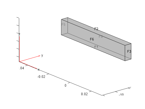
Create an femodel object for transient structural analysis and include the geometry into the model.
model = femodel(AnalysisType="structuralTransient", ...
                Geometry=gm);
Specify Young's modulus, Poisson's ratio, and the mass density of the material.
model.MaterialProperties = ...
    materialProperties(YoungsModulus=210E9, ...
                       PoissonsRatio=0.3, ...
                       MassDensity=7800);
Fix one end of the beam.
model.FaceBC(5) = faceBC(Constraint="fixed");Apply a sinusoidal displacement along the y-direction on the end opposite the fixed end of the beam.
yDisplacementFunc = ...
@(location,state) ones(size(location.y))*1E-4*sin(50*state.time);
model.FaceBC(3) = faceBC(YDisplacement=yDisplacementFunc);
Generate a mesh.
model = generateMesh(model,Hmax=0.01);
Specify the zero initial displacement and velocity.
model.CellIC = cellIC(Displacement=[0;0;0],Velocity=[0;0;0]);
Solve the problem.
tlist = 0:0.002:0.2;
R = solve(model,tlist);
Interpolate the strain at the geometric center of the beam.
coordsMidSpan = [0;0;0.005];
intrpStrain = interpolateStrain(R,coordsMidSpan);
Plot the normal strain at the geometric center of the beam.
plot(R.SolutionTimes,intrpStrain.exx)
title("X-Direction Normal Strain at Beam Center")
Input Arguments
Solution of the structural analysis problem, specified as a StaticStructuralResults, TransientStructuralResults, or FrequencyStructuralResults object. Create
structuralresults by using the solve function.
x-coordinate query points, specified as a real array.
interpolateStrain evaluates the strains at the 2-D
coordinate points [xq(i),yq(i)] or at the 3-D coordinate
points [xq(i),yq(i),zq(i)]. Therefore,
xq, yq, and (if present)
zq must have the same number of entries.
interpolateStrain converts query points to column
vectors xq(:), yq(:), and (if present)
zq(:). The function returns strains as an
FEStruct object with the properties containing
vectors of the same size as these column vectors. To ensure that the
dimensions of the returned solution are consistent with the dimensions of
the original query points, use the reshape function. For
example, use intrpStrain =
reshape(intrpStrain.exx,size(xq)).
Data Types: double
y-coordinate query points, specified as a real array.
interpolateStrain evaluates the strains at the 2-D
coordinate points [xq(i),yq(i)] or at the 3-D coordinate
points [xq(i),yq(i),zq(i)]. Therefore,
xq, yq, and (if present)
zq must have the same number of entries.
Internally, interpolateStrain converts the query points
to the column vector yq(:).
Data Types: double
z-coordinate query points, specified as a real array.
interpolateStrain evaluates the strains at the 3-D
coordinate points [xq(i),yq(i),zq(i)]. Therefore,
xq, yq, and
zq must have the same number of entries. Internally,
interpolateStrain converts the query points to the
column vector zq(:).
Data Types: double
Query points, specified as a real matrix with either two rows for 2-D
geometry or three rows for 3-D geometry. interpolateStrain evaluates the strains at the coordinate
points querypoints(:,i), so each column of
querypoints contains exactly one 2-D or 3-D query
point.
Example: For 2-D geometry, querypoints = [0.5,0.5,0.75,0.75;
1,2,0,0.5]
Data Types: double
Output Arguments
Strains at the query points, returned as an FEStruct
object with the properties representing spatial components of strain at the
query points. For query points that are outside the geometry,
intrpStrain returns NaN.
Properties of an FEStruct object are read-only.
Version History
Introduced in R2017bFor frequency response structural problems, interpolateStrain
interpolates strain for all frequency steps.
For transient structural problems, interpolateStrain
interpolates strain for all time steps.
MATLAB Command
You clicked a link that corresponds to this MATLAB command:
Run the command by entering it in the MATLAB Command Window. Web browsers do not support MATLAB commands.
选择网站
选择网站以获取翻译的可用内容,以及查看当地活动和优惠。根据您的位置,我们建议您选择:。
您也可以从以下列表中选择网站:
如何获得最佳网站性能
选择中国网站(中文或英文)以获得最佳网站性能。其他 MathWorks 国家/地区网站并未针对您所在位置的访问进行优化。
美洲
- América Latina (Español)
- Canada (English)
- United States (English)
欧洲
- Belgium (English)
- Denmark (English)
- Deutschland (Deutsch)
- España (Español)
- Finland (English)
- France (Français)
- Ireland (English)
- Italia (Italiano)
- Luxembourg (English)
- Netherlands (English)
- Norway (English)
- Österreich (Deutsch)
- Portugal (English)
- Sweden (English)
- Switzerland
- United Kingdom (English)