evaluateHeatRate
Evaluate integrated heat flow rate normal to specified boundary
Description
Qn = evaluateHeatRate(thermalresults,RegionType,RegionID)RegionType and RegionID.
Examples
Compute the heat flow rate across a face of the block geometry.
Create an femodel object for steady-state thermal analysis and include a block geometry into the model.
model = femodel(AnalysisType="thermalSteady", ...
                Geometry="Block.stl");
Plot the geometry.
pdegplot(model.Geometry,FaceLabels="on",FaceAlpha=0.5)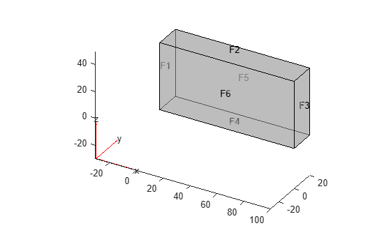
Specify the thermal conductivity of the block.
model.MaterialProperties = ...
    materialProperties(ThermalConductivity=80);
Apply constant temperatures on the opposite ends of the block. All other faces are insulated by default.
model.FaceBC(1) = faceBC(Temperature=100);
model.FaceBC(3) = faceBC(Temperature=50);
Generate a mesh.
model = generateMesh(model);
Solve the thermal problem.
R = solve(model);
Compute the heat flow rate across face 3 of the block.
Qn = evaluateHeatRate(R,Face=3)
Qn =
4.0000e+04
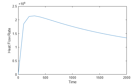
Compute the heat flow rate across the surface of the cooling sphere.
Create an femodel object for transient thermal analysis and include a unit sphere into the model.
model = femodel(AnalysisType="thermalTransient", ...
                Geometry=multisphere(1));
Generate a mesh.
model = generateMesh(model,GeometricOrder="linear");Specify thermal properties of the sphere.
model.MaterialProperties = ...
    materialProperties(ThermalConductivity=80, ...
                       SpecificHeat=460, ...
                       MassDensity=7800);
Apply a convection boundary condition on the surface of the sphere.
model.FaceLoad(1) = ...
    faceLoad(ConvectionCoefficient=500,...
             AmbientTemperature=30);
Set the initial temperature.
model.CellIC = cellIC(Temperature=800);
Solve the thermal problem.
tlist = 0:100:2000;
R = solve(model,tlist);
Compute the heat flow rate across the surface of the sphere over time.
Qn = evaluateHeatRate(R,Face=1);
plot(tlist,Qn)
xlabel("Time")
ylabel("Heat Flow Rate")
Input Arguments
Output Arguments
Version History
Introduced in R2017a