Solve Poisson Equation on Unit Disk Using Physics-Informed Neural Networks

This example uses:

This example shows how to solve the Poisson equation with Dirichlet boundary conditions using a physics-informed neural network (PINN). You generate the required data for training the PINN by using the PDE model setup.

The Poisson equation on a unit disk with zero Dirichlet boundary condition can be written as $- Δ u = 1$ in $Ω$ , $u = 0$ on $δ Ω$ , where $Ω$ is the unit disk. The exact solution is

$u (x, y) = \frac{1 - x^{2} - y^{2}}{4} .$

PDE Model Setup

Create the PDE model and include the geometry.

model = createpde;
geometryFromEdges(model,@circleg);

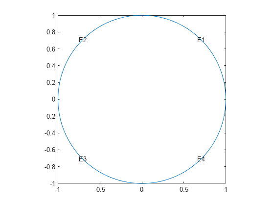
Plot the geometry and display the edge labels for use in the boundary condition definition.

figure 
pdegplot(model,EdgeLabels="on"); 
axis equal

Figure contains an axes object. The axes object contains 5 objects of type line, text.

Specify zero Dirichlet boundary conditions on all edges.

applyBoundaryCondition(model,"dirichlet", ...
    Edge=1:model.Geometry.NumEdges,u=0);

Create a structural array of coefficients. Specify the coefficients for the PDE model.

pdeCoeffs.m = 0;
pdeCoeffs.d = 0;
pdeCoeffs.c = 1;
pdeCoeffs.a = 0;
pdeCoeffs.f = 1;
specifyCoefficients(model,m=pdeCoeffs.m,d=pdeCoeffs.d, ...
    c=pdeCoeffs.c,a=pdeCoeffs.a,f=pdeCoeffs.f);

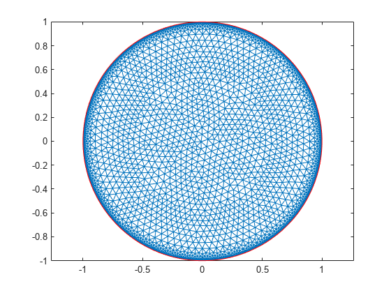
Generate and plot a mesh with a large number of nodes on the boundary.

msh = generateMesh(model,Hmax=0.05,Hgrad=2, ...
    Hedge={1:model.Geometry.NumEdges,0.005});
figure 
pdemesh(model); 
axis equal

Figure contains an axes object. The axes object contains 2 objects of type line.

Generate Spatial Data for Training PINN

To train the PINN, model loss at the collocation points on the domain and boundary. The collocation points in this example are mesh nodes.

boundaryNodes = findNodes(msh,"region", ...
                          Edge=1:model.Geometry.NumEdges);
domainNodes = setdiff(1:size(msh.Nodes,2),boundaryNodes);
domainCollocationPoints = msh.Nodes(:,domainNodes)';

Define Network Architecture

Define a multilayer perceptron architecture with four fully connected operations, each with 50 hidden neurons. The first fully connected operation has two input channels corresponding to the inputs x and y. The last fully connected operation has one output corresponding to u(x,y).

numNeurons = 50;
layers = [
    featureInputLayer(2,Name="featureinput")
    fullyConnectedLayer(numNeurons,Name="fc1")
    tanhLayer(Name="tanh_1")
    fullyConnectedLayer(numNeurons,Name="fc2")
    tanhLayer(Name="tanh_2")
    fullyConnectedLayer(numNeurons,Name="fc3")
    tanhLayer(Name="tanh_3")
    fullyConnectedLayer(1,Name="fc4")
    ];

pinn = dlnetwork(layers);

Specify Training Options

Specify the number of epochs, mini-batch size, initial learning rate, and the learning rate decay.

numEpochs = 50;
miniBatchSize = 500;
initialLearnRate = 0.01;
learnRateDecay = 0.005;

Convert the training data to dlarray (Deep Learning Toolbox) objects.

ds = arrayDatastore(domainCollocationPoints);
mbq = minibatchqueue(ds,MiniBatchSize=miniBatchSize, ...
                        MiniBatchFormat="BC");

Initialize the average gradients and squared average gradients.

averageGrad = [];
averageSqGrad = [];

Calculate the total number of iterations for the training progress monitor.

numIterations = numEpochs* ...
    ceil(size(domainCollocationPoints,1)/miniBatchSize);

Initialize the trainingProgressMonitor (Deep Learning Toolbox) object.

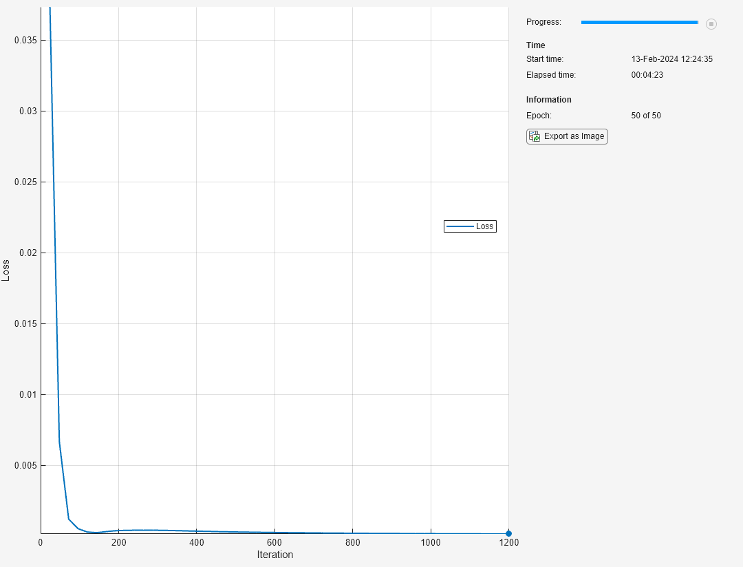
monitor = trainingProgressMonitor(Metrics="Loss", ...
                                  Info="Epoch", ...
                                  XLabel="Iteration");

Training Progress window. The figure is set to track the loss with respect to the learnable parameters in pinn.

Train PINN

Train the model using a custom training loop. Update the network parameters using the adamupdate (Deep Learning Toolbox) function. At the end of each iteration, display the training progress.

This training code uses the modelLoss helper function. For more information, see Model Loss Function.

iteration = 0;
epoch = 0;
learningRate = initialLearnRate;
while epoch < numEpochs && ~monitor.Stop
    epoch = epoch + 1;
    reset(mbq);
    while hasdata(mbq) && ~monitor.Stop
        iteration = iteration + 1;
        XY = next(mbq);
        % Evaluate the model loss and gradients using dlfeval.
        [loss,gradients] = dlfeval(@modelLoss,model,pinn,XY,pdeCoeffs);
        % Update the network parameters using the adamupdate function.
        [pinn,averageGrad,averageSqGrad] = ...
            adamupdate(pinn,gradients,averageGrad, ...
                       averageSqGrad,iteration,learningRate);
    end
    % Update learning rate.
    learningRate = initialLearnRate / (1+learnRateDecay*iteration);
    % Update the training progress monitor.
    recordMetrics(monitor,iteration,Loss=loss);
    updateInfo(monitor,Epoch=epoch + " of " + numEpochs);
    monitor.Progress = 100 * iteration/numIterations;
end

Test PINN

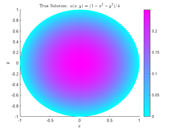
Find and plot the true solution at the mesh nodes.

trueSolution = @(msh) (1-msh.Nodes(1,:).^2-msh.Nodes(2,:).^2)/4;
Utrue = trueSolution(msh);

figure;
pdeplot(model,XYData=Utrue);
xlabel('$x$',interpreter='latex')
ylabel('$y$',interpreter='latex')
zlabel('$u(x,y)$',interpreter='latex')
title('True Solution: $u(x,y) = (1-x^2-y^2)/4$', ...
                      interpreter='latex')

Figure contains an axes object. The axes object with title True Solution: u leftParenthesis x , y rightParenthesis equals leftParenthesis 1 minus x Squared baseline minus y Squared baseline rightParenthesis slash 4, xlabel $x$, ylabel $y$ contains an object of type patch.

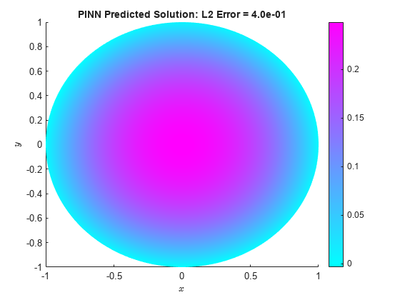
Now find and plot the solution predicted by the PINN.

nodesDLarry = dlarray(msh.Nodes,"CB");
Upinn = gather(extractdata(predict(pinn,nodesDLarry)));

figure;
pdeplot(model,XYData=Upinn);
xlabel('$x$',interpreter='latex')
ylabel('$y$',interpreter='latex')
zlabel('$u(x,y)$',interpreter='latex')
title(sprintf(['PINN Predicted Solution: ' ...
    'L2 Error = %0.1e'],norm(Upinn-Utrue)))

Figure contains an axes object. The axes object with title PINN Predicted Solution: L2 Error = 1.8e-01, xlabel $x$, ylabel $y$ contains an object of type patch.

Model Loss Function

The modelLoss helper function takes as inputs a dlnetwork object pinn and a mini-batch of input data XY. The function returns the loss and the gradients of the loss with respect to the learnable parameters in pinn. To compute the gradients automatically, use the dlgradient (Deep Learning Toolbox) function. Train the model by enforcing that, given an input (x,y), the output of the network u(x,y) fulfills the Poisson equation and the boundary conditions.

function [loss,gradients] = modelLoss(model,net,XY,pdeCoeffs)
dim = 2;
[U,~] = forward(net,XY);

% Compute gradients of U and Laplacian of U.
gradU = dlgradient(sum(U,"all"),XY,EnableHigherDerivatives=true);
Laplacian = 0;
for i=1:dim
    gradU2 = dlgradient(sum(pdeCoeffs.c.*gradU(i,:),"all"), ...
                          XY,EnableHigherDerivatives=true);
    Laplacian = gradU2(i,:)+Laplacian;
end

% Enforce PDE. Calculate lossF.
res = -pdeCoeffs.f - Laplacian + pdeCoeffs.a.*U;
zeroTarget = zeros(size(res),"like",res);
lossF = mse(res,zeroTarget);

% Enforce boundary conditions. Calculate lossU.
actualBC = []; % Boundary information
BC_XY = []; % Boundary coordinates
% Loop over the boundary edges and find boundary
% coordinates and actual BC assigned to PDE model.
numBoundaries = model.Geometry.NumEdges;
for i=1:numBoundaries
    BCi = findBoundaryConditions(model.BoundaryConditions,Edge=i);
    BCiNodes = findNodes(model.Mesh,"region",Edge=i);
    BC_XY = [BC_XY,model.Mesh.Nodes(:,BCiNodes)]; %#ok<AGROW> 
    actualBCi = ones(1,numel(BCiNodes))*BCi.u;
    actualBC = [actualBC actualBCi]; %#ok<AGROW>
end
BC_XY = dlarray(BC_XY,"CB"); % Format the coordinates
[predictedBC,~] = forward(net,BC_XY);
lossU = mse(predictedBC,actualBC);

% Combine the losses. Use a weighted linear combination 
% of loss (lossF and lossU) terms.
lambda = 0.4; % Weighting factor
loss = lambda*lossF + (1-lambda)*lossU;

% Calculate gradients with respect to the learnable parameters.
gradients = dlgradient(loss,net.Learnables); 
end