Main Content

gaspl

RF signal attenuation due to atmosphere gaseous absorption

Description

L = gaspl(range,freq,T,P,den) returns the signal attenuation, L, due to atmosphere gaseous absorption.

  • range represents the signal path length.

  • freq represents the signal carrier frequency.

  • T represents the ambient temperature.

  • P represents the atmospheric pressure.

  • den represents the atmospheric water vapor density.

The gaspl function applies the International Telecommunication Union (ITU) atmospheric gas attenuation model [1] to calculate path loss for signals primarily due to oxygen and water vapor. The model computes attenuation as a function of ambient temperature, pressure, water vapor density, and signal frequency.

The function requires that the signal path is contained entirely in a homogeneous environment – temperature T, atmospheric pressure P, and water vapor density den do not vary along the signal path. You can account for the variation of atmospheric parameters with height using the tropopl and atmositu functions in the Radar Toolbox.

The attenuation model applies only for frequencies at 1–1000 GHz.

example

Examples

collapse all

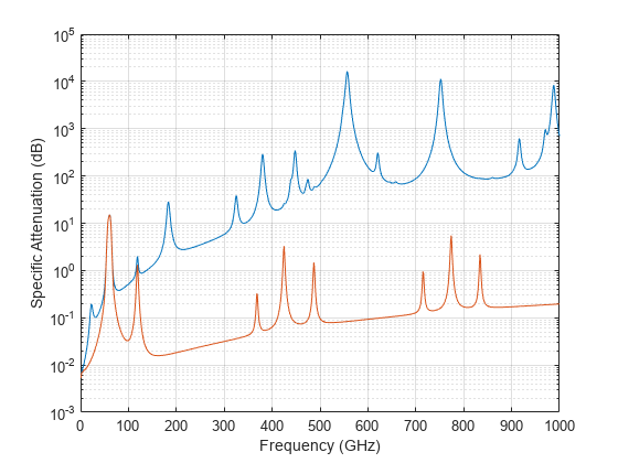
Compute the attenuation spectrum from 1 to 1000 GHz for an atmospheric pressure of 101.300 kPa and a temperature of 15C. Plot the spectrum for a water vapor density of 7.5 g/m3 and then plot the spectrum for dry air (zero water vapor density).

Set the attenuation frequencies.

freq = [1:1000]*1e9;

Assume a 1 km path distance.

R = 1000.0;

Compute the attenuation for air containing water vapor.

T = 15;
P = 101300.0;
W = 7.5;
L = gaspl(R,freq,T,P,W);

Compute the attenuation for dry air.

L0 = gaspl(R,freq,T,P,0.0);

Plot the attenuations.

semilogy(freq/1e9,L)
hold on
semilogy(freq/1e9,L0)
grid
xlabel('Frequency (GHz)')
ylabel('Specific Attenuation (dB)')
hold off

Figure contains an axes object. The axes object with xlabel Frequency (GHz), ylabel Specific Attenuation (dB) contains 2 objects of type line.

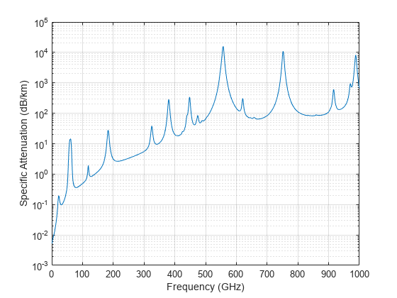
First, plot the specific attenuation of atmospheric gases for frequencies from 1 GHz to 1000 GHz. Assume a sea-level dry air pressure of 101.325e5 kPa and a water vapor density of 7.5 g/m3. The air temperature is 20C. Specific attenuation is defined as dB loss per kilometer. Then, plot the actual attenuation at 10 GHz for a span of ranges.

Plot Specific Atmospheric Gas Attenuation

Set the atmosphere temperature, pressure, water vapor density.

T = 20.0;
Patm = 101.325e3;
rho_wv = 7.5;

Set the propagation distance, speed of light, and frequencies.

km = 1000.0;
c = physconst('LightSpeed');
freqs = [1:1000]*1e9;

Compute and plot the atmospheric gas loss.

loss = gaspl(km,freqs,T,Patm,rho_wv);
semilogy(freqs/1e9,loss)
grid on
xlabel('Frequency (GHz)')
ylabel('Specific Attenuation (dB/km)')

Figure contains an axes object. The axes object with xlabel Frequency (GHz), ylabel Specific Attenuation (dB/km) contains an object of type line.

Plot Actual Atmospheric and Free Space Attenuation

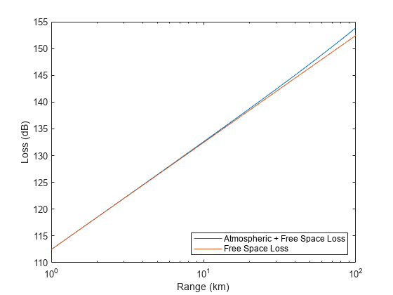
Compute both free space loss and atmospheric gas loss at 10 GHz for ranges from 1 to 100 km. The frequency corresponds to an X-band radar. Then, plot the free space loss and the total (atmospheric + free space) loss.

ranges = [1:100]*1000;
freq_xband = 10e9;
loss_gas = gaspl(ranges,freq_xband,T,Patm,rho_wv);
lambda = c/freq_xband;
loss_fsp = fspl(ranges,lambda);
semilogx(ranges/1000,loss_gas + loss_fsp.',ranges/1000,loss_fsp)
legend('Atmospheric + Free Space Loss','Free Space Loss','Location','SouthEast')
xlabel('Range (km)')
ylabel('Loss (dB)')

Figure contains an axes object. The axes object with xlabel Range (km), ylabel Loss (dB) contains 2 objects of type line. These objects represent Atmospheric + Free Space Loss, Free Space Loss.

Input Arguments

collapse all

Signal path length, in meters, used to compute attenuation, specified as a nonnegative real-valued scalar or vector. You can specify multiple path lengths simultaneously.

Example: [13000.0,14000.0]

Signal frequency in Hz, specified as a positive real-valued scalar, or as an N-by-1 nonnegative real-valued vector or 1-by-N nonnegative real-valued vector. You can specify multiple frequencies simultaneously. Frequencies must lie in the range 1–1000 GHz.

Example: [1.4e9,2.0e9]

Ambient temperature in °C, specified as a real-valued scalar.

Example: -10.0

Dry air pressure in Pa, specified as a positive real-valued scalar. One standard atmosphere at sea level is 101325 Pa.

Example: 101300.0

Water vapor density or absolute humidity, in g/m3, specified as a nonnegative real-valued scalar. The maximum water vapor density of air at 30° C is approximately 30.0 g/m3. The maximum water vapor density of air at 0°C is approximately 5.0 g/m3.

Example: 4.0

Output Arguments

collapse all

Signal attenuation in dB, returned as a real-valued M-by-N matrix. Each matrix row represents a different path where M is the number of paths. Each column represents a different frequency where N is the number of frequencies.

More About

collapse all

Atmospheric Gas Attenuation Model

This model calculates the attenuation of signals that propagate through atmospheric gases.

Electromagnetic signals attenuate when they propagate through the atmosphere. This effect is due primarily to the absorption resonance lines of oxygen and water vapor, with smaller contributions coming from nitrogen gas. The model also includes a continuous absorption spectrum below 10 GHz. The ITU model Recommendation ITU-R P.676-10: Attenuation by atmospheric gases is used. The model computes the specific attenuation (attenuation per kilometer) as a function of temperature, pressure, water vapor density, and signal frequency. The atmospheric gas model is valid for frequencies from 1–1000 GHz and applies to polarized and nonpolarized fields.

The formula for specific attenuation at each frequency is

γ=γo(f)+γw(f)=0.1820fN(f).

The quantity N"() is the imaginary part of the complex atmospheric refractivity and consists of a spectral line component and a continuous component:

N(f)=iSiFi+ND(f)

The spectral component consists of a sum of discrete spectrum terms composed of a localized frequency bandwidth function, F(f)i, multiplied by a spectral line strength, Si. For atmospheric oxygen, each spectral line strength is

Si=a1×107(300T)3exp[a2(1(300T)]P.

For atmospheric water vapor, each spectral line strength is

Si=b1×101(300T)3.5exp[b2(1(300T)]W.

P is the dry air pressure, W is the water vapor partial pressure, and T is the ambient temperature. Pressure units are in hectoPascals (hPa) and temperature is in degrees Kelvin. The water vapor partial pressure, W, is related to the water vapor density, ρ, by

W=ρT216.7.

The total atmospheric pressure is P + W.

For each oxygen line, Si depends on two parameters, a1 and a2. Similarly, each water vapor line depends on two parameters, b1 and b2. The ITU documentation cited at the end of this section contains tabulations of these parameters as functions of frequency.

The localized frequency bandwidth functions Fi(f) are complicated functions of frequency described in the ITU references cited below. The functions depend on empirical model parameters that are also tabulated in the reference.

This model applies to both narrowband and wideband atmospheric attenuation. To compute the total attenuation for narrowband signals along a path, the function multiplies the specific attenuation by the path length, R. Then, the total attenuation is Lg= R(γo + γw). To apply the attenuation model to wideband signals, first, divide the wideband signal into frequency subbands, and apply attenuation to each subband. Then, sum all attenuated subband signals into the total attenuated signal.

References

[1] Radiocommunication Sector of International Telecommunication Union. Recommendation ITU-R P.676-10: Attenuation by atmospheric gases 2013.

Extended Capabilities

Version History

Introduced in R2016a