rainpl
RF signal attenuation due to rainfall using ITU model
Syntax
Description
L = rainpl(range,freq,rainrate)L, due to rain with a long-term
statistical rain rate. In this syntax, attenuation is a function of signal path
length, range, signal frequency, freq, and
rain rate, rainrate. The path elevation angle and polarization
tilt angles are assumed to be zero.
The rainpl function applies the International
Telecommunication Union (ITU) rainfall attenuation model to calculate
path loss of signals propagating in a region of rainfall [1]. The function applies when the signal
path is contained entirely in a uniform rainfall environment. Rain
rate does not vary along the signal path. The attenuation model applies
only for frequencies at 1–1000 GHz.
Examples
Compute the signal attenuation due to rainfall for a 20 GHz signal over a distance of 10 km in light and heavy rain.
Propagate the signal in a light rainfall of 1 mm/hr.
rr = 1.0;
L = rainpl(10000,20.0e9,rr)
L =
1.3009
Propagate the signal in a heavy rainfall of 10 mm/hr.
rr = 10.0;
L = rainpl(10000,20.0e9,rr)
L =
8.1584
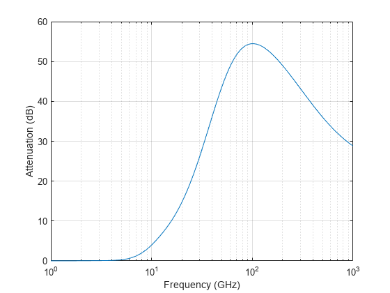
Plot the signal attenuation due to a 20 mm/hr statistical rainfall for signals in the frequency range from 1 to 1000 GHz. The path distance is 10 km.
rr = 20.0;
freq = [1:1000]*1e9;
L = rainpl(10000,freq,rr);
semilogx(freq/1e9,L)
grid
xlabel('Frequency (GHz)')
ylabel('Attenuation (dB)')
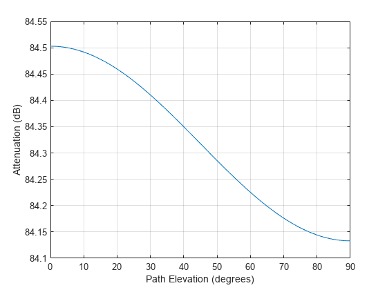
Compute the signal attenuation due to heavy rain as a function of elevation angle. Elevation angles vary from 0 to 90 degrees. Assume a path distance of 100 km and a signal frequency of 100 GHz.
Set the rain rate to 10 mm/hr.
rr = 10.0;
Set the elevation angles, frequency, range.
elev = [0:1:90];
freq = 100.0e9;
rng = 100000.0*ones(size(elev));
Compute and plot the loss.
L = rainpl(rng,freq,rr,elev);
plot(elev,L)
grid
xlabel('Path Elevation (degrees)')
ylabel('Attenuation (dB)')
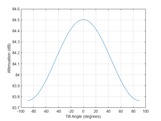
Compute the signal attenuation due to heavy rainfall as a function of the polarization tilt angle. Assume a path distance of 100 km, a signal frequency of 100 GHz, and a path elevation angle of 0 degrees. Set the rainfall rate to 10 mm/hour. Plot the signal attenuation versus polarization tilt angle.
Set the polarization tilt angle to vary from -90 to 90 degrees.
tau = -90:90;
Set the elevation angle, frequency, path distance, and rain rate.
elev = 0;
freq = 100.0e9;
rng = 100e3*ones(size(tau));
rr = 10.0;
Compute and plot the attenuation.
L = rainpl(rng,freq,rr,elev,tau);
plot(tau,L)
grid
xlabel('Tilt Angle (degrees)')
ylabel('Attenuation (dB)')
Input Arguments
Output Arguments
More About
References
[1] Radiocommunication Sector of International Telecommunication Union. Recommendation ITU-R P.838-3: Specific attenuation model for rain for use in prediction methods. 2005.
[2] Radiocommunication Sector of International Telecommunication Union. Recommendation ITU-R P.530-18: Propagation data and prediction methods required for the design of terrestrial line-of-sight systems. 2021.
[3] Recommendation ITU-R P.838-3: Characteristics of precipitation for propagation modelling. 2005
[4] Seybold, J. Introduction to RF Propagation. New York: Wiley & Sons, 2005.
Extended Capabilities
Version History
Introduced in R2016a
See Also
fspl | gaspl | fogpl | cranerainpl | LOSChannel | WidebandLOSChannel