pattern

System object: phased.HeterogeneousURA
Namespace: phased

Plot heterogeneous URA directivity and power pattern

Syntax

pattern(sArray,FREQ) pattern(sArray,FREQ,AZ) pattern(sArray,FREQ,AZ,EL) pattern(___,Name,Value) [PAT,AZ_ANG,EL_ANG] = pattern(___)

Description

pattern(sArray,FREQ) plots the 3-D array directivity pattern (in dBi) for the array specified in sArray. The operating frequency is specified in FREQ.

The integration used when computing array directivity has a minimum sampling grid of 0.1 degrees. If an array pattern has a beamwidth smaller than this, the directivity value will be inaccurate.

pattern(sArray,FREQ,AZ) plots the array directivity pattern at the specified azimuth angle.

pattern(sArray,FREQ,AZ,EL) plots the array directivity pattern at specified azimuth and elevation angles.

pattern(___,Name,Value) plots the array pattern with additional options specified by one or more Name,Value pair arguments.

[PAT,AZ_ANG,EL_ANG] = pattern(___) returns the array pattern in PAT. The AZ_ANG output contains the coordinate values corresponding to the rows of PAT. The EL_ANG output contains the coordinate values corresponding to the columns of PAT. If the 'CoordinateSystem' parameter is set to 'uv', then AZ_ANG contains the U coordinates of the pattern and EL_ANG contains the V coordinates of the pattern. Otherwise, they are in angular units in degrees. UV units are dimensionless.

Note

When you need to compute array or element directivity, you can either set the Type property to "directivity" in the pattern object function or use the directivity object function. For a small number of angular directions, it may be more computationally efficient to use the directivity object function. The pattern object function is more efficient for computing directivity for larger angular regions.

Input Arguments

expand all

`sArray` — Heterogeneous URA
System object™

Heterogeneous conformal array, specified as a phased.HeterogeneousURA System object.

Example: sArray= phased.HeterogeneousURA;

`FREQ` — Frequency for computing directivity and patterns
positive scalar | 1-by-L real-valued row vector

Frequencies for computing directivity and patterns, specified as a positive scalar or 1-by-L real-valued row vector. Frequency units are in hertz.

For an antenna, microphone, or sonar hydrophone or projector element, FREQ must lie within the range of values specified by the FrequencyRange or FrequencyVector property of the element. Otherwise, the element produces no response and the directivity is returned as –Inf. Most elements use the FrequencyRange property except for phased.CustomAntennaElement and phased.CustomMicrophoneElement, which use the FrequencyVector property.
For an array of elements, FREQ must lie within the frequency range of the elements that make up the array. Otherwise, the array produces no response and the directivity is returned as –Inf.

Example: [1e8 2e6]

Data Types: double

`AZ` — Azimuth angles
`[-180:180]` (default) | 1-by-N real-valued row vector

Azimuth angles for computing directivity and pattern, specified as a 1-by-N real-valued row vector where N is the number of azimuth angles. Angle units are in degrees. Azimuth angles must lie between –180° and 180°.

The azimuth angle is the angle between the x-axis and the projection of the direction vector onto the xy plane. When measured from the x-axis toward the y-axis, this angle is positive.

Example: [-45:2:45]

Data Types: double

`EL` — Elevation angles
`[-90:90]` (default) | 1-by-M real-valued row vector

Elevation angles for computing directivity and pattern, specified as a 1-by-M real-valued row vector where M is the number of desired elevation directions. Angle units are in degrees. The elevation angle must lie between –90° and 90°.

The elevation angle is the angle between the direction vector and xy-plane. The elevation angle is positive when measured towards the z-axis.

Example: [-75:1:70]

Data Types: double

Name-Value Arguments

expand all

Specify optional pairs of arguments as Name1=Value1,...,NameN=ValueN, where Name is the argument name and Value is the corresponding value. Name-value arguments must appear after other arguments, but the order of the pairs does not matter.

Before R2021a, use commas to separate each name and value, and enclose Name in quotes.

`CoordinateSystem` — Plotting coordinate system
`"polar"` (default) | `"rectangular"` | `"uv"`

Plotting coordinate system of the pattern, specified as the comma-separated pair consisting of CoordinateSystem and one of "polar", "rectangular", or "uv". When CoordinateSystem is set to "polar" or "rectangular", the AZ and EL arguments specify the pattern azimuth and elevation, respectively. AZ values must lie between –180° and 180°. EL values must lie between –90° and 90°. If CoordinateSystem is set to "uv", AZ and EL then specify U and V coordinates, respectively. AZ and EL must lie between -1 and 1.

Example: "uv"

Data Types: char

`Type` — Displayed pattern type
`"directivity"` (default) | `"efield"` | `"power"` | `"powerdb"`

Displayed pattern type, specified as the equal-sign-separated pair consisting of Type and one of

"directivity" — directivity pattern measured in dBi.
"efield" — field pattern of the sensor or array. For acoustic sensors, the displayed pattern is for the scalar sound field.
"power" — power pattern of the sensor or array defined as the square of the field pattern.
"powerdb" — power pattern converted to dB.

Example: "powerdb"

Data Types: char

`Orientation` — Array orientation
`[0;0;0]`. (default) | 3-by-1 real-valued column vector

Array orientation, specified as a 3-by-1 real-valued column vector containing three rotation angles. The three angles define orthogonal rotations with respect to the x-, y-, and z-axes of the local coordinate system. To create the full orientation matrix, the orthogonal rotations are applied in this order:

a rotation around the positive x-axis by the angle θ_x.
a rotation around the positive y-axis by the angle θ_y.
a rotation around the positive z-axis by the angle θ_z.

Positive angles are defined using the right-handed rule. A positive angle defines a rotation that appears clockwise when looking towards the positive direction of the axis, and negative values when the rotation appears counter-clockwise. The right-hand rule is invoked by pointing the right-hand thumb along an axis. Then the other fingers of the right hand curl in the positive direction,

`Normalize` — Display normalize pattern
`true` (default) | `false`

Display normalized pattern, specified as the comma-separated pair consisting of Normalize and a Boolean. Set this parameter to true to display a normalized pattern. This parameter does not apply when you set Type to "directivity". Directivity patterns are already normalized.

Data Types: logical

`ShowArray` — View array geometry
`false` (default) | `true`

View the array geometry along with the 3D radiation pattern, specified as false or true.

Data Types: logical

`ShowLocalCoordinates` — Show local coordinate axes
`true` (default) | `false`

Show the local coordinate axes, specified as true or false.

Data Types: logical

`ShowColorbar` — Show colorbar
`true` (default) | `false`

Show the colorbar, specified as true or false.

Data Types: logical

`Parent` — Handle to axis
scalar

Handle to the axes along which the array geometry is displayed specified as a scalar.

`PlotStyle` — Plotting style
`"overlay"` (default) | `"waterfall"`

Plotting style, specified as the equal-sign-separated pair consisting of Plotstyle and either "overlay" or "waterfall". This parameter applies when you specify multiple frequencies in FREQ in 2-D plots. You can draw 2-D plots by setting one of the arguments AZ or EL to a scalar.

Data Types: char

`Polarization` — Polarized field component
`'combined'` (default) | `'H'` | `'V'`

Polarized field component to display, specified as the comma-separated pair consisting of 'Polarization' and 'combined', 'H', or 'V'. This parameter applies only when the sensors are polarization-capable and when the 'Type' parameter is not set to 'directivity'. This table shows the meaning of the display options.

`'Polarization'`	Display
`'combined'`	Combined H and V polarization components
`'H'`	H polarization component
`'V'`	V polarization component

Example: 'V'

Data Types: char

`PropagationSpeed` — Signal propagation speed
speed of light (default) | positive scalar

Signal propagation speed, specified as the comma-separated pair consisting of PropagationSpeed and a positive scalar in meters per second.

Example: PropagationSpeed="physconst('LightSpeed')"

Data Types: double

`Weights` — Array weights
1 (default) | N-by-1 complex-valued column vector | N-by-L complex-valued matrix

Array weights, specified as the comma-separated pair consisting of 'Weights' and an N-by-1 complex-valued column vector or N-by-L complex-valued matrix. Array weights are applied to the elements of the array to produce array steering, tapering, or both. The dimension N is the number of elements in the array. The dimension L is the number of frequencies specified by FREQ.

Weights Dimension	FREQ Dimension	Purpose
N-by-1 complex-valued column vector	Scalar or 1-by-L row vector	Applies a set of weights for the single frequency or for all L frequencies.
N-by-L complex-valued matrix	1-by-L row vector	Applies each of the L columns of `'Weights'` for the corresponding frequency in `FREQ`.

Note

Use complex weights to steer the array response toward different directions. You can create weights using the phased.SteeringVector System object or you can compute your own weights. In general, you apply Hermitian conjugation before using weights in any Phased Array System Toolbox™ function or System object such as phased.Radiator or phased.Collector. However, for the directivity, pattern, patternAzimuth, and patternElevation methods of any array System object use the steering vector without conjugation.

Example: 'Weights',ones(N,M)

Data Types: double
Complex Number Support: Yes

Output Arguments

expand all

`PAT` — Array pattern
M-by-N real-valued matrix

Array pattern, returned as an M-by-N real-valued matrix. The dimensions of PAT correspond to the dimensions of the output arguments AZ_ANG and EL_ANG.

`AZ_ANG` — Azimuth angles
scalar | 1-by-N real-valued row vector

Azimuth angles for displaying directivity or response pattern, returned as a scalar or 1-by-N real-valued row vector corresponding to the dimension set in AZ. The columns of PAT correspond to the values in AZ_ANG. Units are in degrees.

`EL_ANG` — Elevation angles
scalar | 1-by-M real-valued row vector

Elevation angles for displaying directivity or response, returned as a scalar or 1-by-M real-valued row vector corresponding to the dimension set in EL. The rows of PAT correspond to the values in EL_ANG. Units are in degrees.

Examples

expand all

Azimuth Pattern and Directivity of Heterogeneous URA

Open Live Script

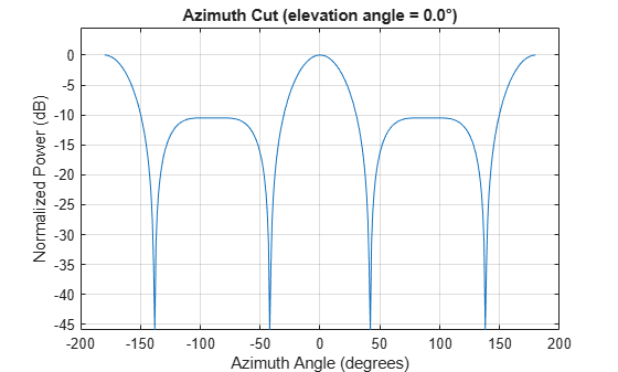
Construct a 3-by-3 heterogeneous URA of short-dipole antenna elements with a rectangular lattice. Then, plot the array's azimuth pattern at 300 MHz.

sElement1 = phased.ShortDipoleAntennaElement(...
    'FrequencyRange',[2e8 5e8],...
    'AxisDirection','Z');
sElement2 = phased.ShortDipoleAntennaElement(...
    'FrequencyRange',[2e8 5e8],...
    'AxisDirection','Y');
sArray = phased.HeterogeneousURA(...
    'ElementSet',{sElement1,sElement2},...
    'ElementIndices',[1 1 1; 2 2 2; 1 1 1]);
fc = 300e6;
c = physconst('LightSpeed');
pattern(sArray,fc,[-180:180],0,...
    'PropagationSpeed',c,...
    'CoordinateSystem','rectangular',...
    'Type','powerdb',...
    'Normalize',true,...
    'Polarization','combined')

Figure contains an axes object. The axes object with title Azimuth Cut (elevation angle = 0.0°), xlabel Azimuth Angle (degrees), ylabel Normalized Power (dB) contains an object of type line. This object represents 300 MHz.

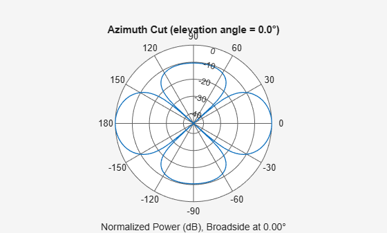
Plot the same result in polar form.

pattern(sArray,fc,[-180:180],0,...
    'PropagationSpeed',c,...
    'CoordinateSystem','polar',...
    'Type','powerdb',...
    'Normalize',true,...
    'Polarization','combined')

Figure contains an axes object. The hidden axes object contains 3 objects of type line, text. This object represents 300 MHz .

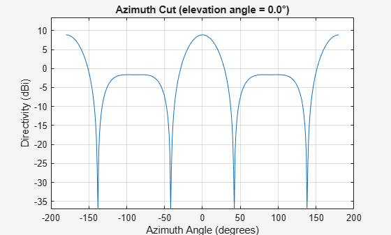
Finally, plot the directivity.

pattern(sArray,fc,[-180:180],0,...
    'PropagationSpeed',c,...
    'CoordinateSystem','rectangular',...
    'Type','directivity')

Figure contains an axes object. The axes object with title Azimuth Cut (elevation angle = 0.0°), xlabel Azimuth Angle (degrees), ylabel Directivity (dBi) contains an object of type line. This object represents 300 MHz.

Azimuth Pattern of Heterogeneous URA for Two Sets of Weights

Open Live Script

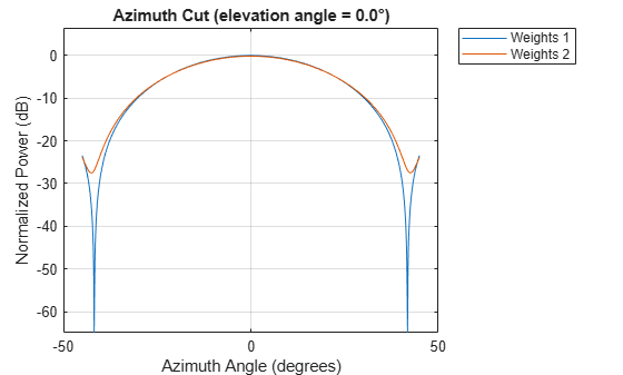
Construct a square 3-by-3 heterogeneous URA composed of 9 short-dipole antenna elements with different orientations. Plot the array azimuth pattern from -45 degrees to 45 degrees in 0.1 degree increments. The Weights parameter lets you display the array pattern simultaneously for different sets of weights: in this case a uniform set of weights and a tapered set.

sElement1 = phased.ShortDipoleAntennaElement(...
    'FrequencyRange',[2e8 5e8],...
    'AxisDirection','Z');
sElement2 = phased.ShortDipoleAntennaElement(...
    'FrequencyRange',[2e8 5e8],...
    'AxisDirection','Y');
sArray = phased.HeterogeneousURA(...
    'ElementSet',{sElement1,sElement2},...
    'ElementIndices',[1 1 1; 2 2 2; 1 1 1]);
fc = [3e8];
c = physconst('LightSpeed');
wts1 = ones(9,1)/9;
wts2 = [.7,.7,.7,.7,1,.7,.7,.7,.7]';
wts2 = wts2/sum(wts2);
pattern(sArray,fc,[-45:0.1:45],0,...
    'PropagationSpeed',c,...
    'CoordinateSystem','rectangular',...
    'Type','powerdb',...
    'Weights',[wts1,wts2],...
    'Polarization','combined')

Figure contains an axes object. The axes object with title Azimuth Cut (elevation angle = 0.0°), xlabel Azimuth Angle (degrees), ylabel Normalized Power (dB) contains 2 objects of type line. These objects represent Weights 1, Weights 2.

More About

expand all

Directivity

Directivity describes the directionality of the radiation pattern of a sensor element or array of sensor elements.

Higher directivity is desired when you want to transmit more radiation in a specific direction. Directivity is the ratio of the transmitted radiant intensity in a specified direction to the radiant intensity transmitted by an isotropic radiator with the same total transmitted power

$D = 4 π \frac{U_{rad} (θ, φ)}{P_{total}}$

where U_rad(θ,φ) is the radiant intensity of a transmitter in the direction (θ,φ) and P_total is the total power transmitted by an isotropic radiator. For a receiving element or array, directivity measures the sensitivity toward radiation arriving from a specific direction. The principle of reciprocity shows that the directivity of an element or array used for reception equals the directivity of the same element or array used for transmission. When converted to decibels, the directivity is denoted as dBi. For information on directivity, read the notes on Element Directivity and Array Directivity.

Convert plotResponse to pattern

For antenna, microphone, and array System objects, the pattern method replaces the plotResponse method. In addition, two new simplified methods exist just to draw 2-D azimuth and elevation pattern plots. These methods are patternAzimuth and patternElevation.

The following table is a guide for converting your code from using plotResponse to pattern. Notice that some of the inputs have changed from input arguments to Name-Value pairs and conversely. The general pattern method syntax is

pattern(H,FREQ,AZ,EL,'Name1','Value1',...,'NameN','ValueN')

plotResponse Inputs plotResponse Description pattern Inputs

H argument Antenna, microphone, or array System object. H argument (no change)

FREQ argument Operating frequency. FREQ argument (no change)

V argument Propagation speed. This argument is used only for arrays. 'PropagationSpeed' name-value pair. This parameter is only used for arrays.

'Format' and 'RespCut' name-value pairs

These options work together to let you create a plot in angle space (line or polar style) or UV space. They also determine whether the plot is 2-D or 3-D. This table shows you how to create different types of plots using plotResponse.

Display space
Angle space (2D)	Set `'RespCut' to 'Az' or 'El'`. Set `'Format'` to `'line'` or `'polar'`. Set the display axis using either the `'AzimuthAngles'` or `'ElevationAngles'` name-value pairs.
Angle space (3D)	Set `'RespCut'` to `'3D'`. Set `'Format'` to `'line'` or `'polar'`. Set the display axis using both the `'AzimuthAngles'` and`'ElevationAngles'` name-value pairs.
UV space (2D)	Set `'RespCut'` to`'U'`. Set `'Format'` to `'UV'`. Set the display range using the `'UGrid'` name-value pair.
UV space (3D)	Set `'RespCut'` to`'3D'`. Set `'Format'` to `'UV'`. Set the display range using both the `'UGrid'` and `'VGrid'` name-value pairs.

'CoordinateSystem' name-value pair used together with the AZ and EL input arguments.

'CoordinateSystem' has the same options as the plotResponse method 'Format'name-value pair, except that 'line' is now named 'rectangular'. The table shows how to create different types of plots using pattern.

Display space
Angle space (2D)	Set `'Coordinate System'` to `'rectangular'` or `'polar'`. Specify either `AZ` or `EL` as a scalar.
Angle space (3D)	Set `'Coordinate System'` to `'rectangular'` or `'polar'`. Specify both `AZ` and `EL` as vectors.
UV space (2D)	Set `'Coordinate System'` to `'uv'`. Use `AZ` to specify a U-space vector. Use `EL` to specify a V-space scalar.
UV space (3D)	Set `'Coordinate System'` to `'uv'`. Use `AZ` to specify a U-space vector. Use `EL` to specify a V-space vector.

If you set CoordinateSystem to 'uv', enter the UV grid values using AZ and EL.

'CutAngle' name-value pair Constant angle at to take an azimuth or elevation cut. When producing a 2-D plot and when 'RespCut' is set to 'Az' or 'El', use 'CutAngle' to set the slice across which to view the plot. No equivalent name-value pair. To create a cut, specify either AZ or EL as a scalar, not a vector.

'NormalizeResponse' name-value pair

Normalizes the plot. When 'Unit' is set to 'dbi', you cannot specify 'NormalizeResponse'.

Use the 'Normalize' name-value pair. When 'Type' is set to 'directivity' you cannot specify 'Normalize'.

'OverlayFreq' name-value pair

Plot multiple frequencies on the same 2-D plot. Available only when 'Format' is set to 'line' or 'uv' and 'RespCut' is not set to '3D'. The value true produces an overlay plot and the value false produces a waterfall plot.

'PlotStyle' name-value pair plots multiple frequencies on the same 2-D plot.

The values 'overlay' and 'waterfall' correspond to 'OverlayFreq' values of true and false. The option 'waterfall' is allowed only when 'CoordinateSystem' is set to 'rectangular' or 'uv'.

'Polarization' name-value pair Determines how to plot polarized fields. Options are 'None', 'Combined', 'H', or 'V'. 'Polarization' name-value pair determines how to plot polarized fields. The 'None' option is removed. The options 'Combined', 'H', or 'V' are unchanged.

'Unit' name-value pair

Determines the plot units. Choose 'db', 'mag', 'pow', or 'dbi', where the default is 'db'.

'Type' name-value pair, uses equivalent options with different names

`plotResponse`	`pattern`
`'db'`	`'powerdb'`
`'mag'`	`'efield'`
`'pow'`	`'power'`
`'dbi'`	`'directivity'`

'Weights' name-value pair Array element tapers (or weights). 'Weights' name-value pair (no change).

'AzimuthAngles' name-value pair

Azimuth angles used to display the antenna or array response.

AZ argument

'ElevationAngles' name-value pair

Elevation angles used to display the antenna or array response.

EL argument

'UGrid' name-value pair

Contains U coordinates in UV-space.

AZ argument when 'CoordinateSystem' name-value pair is set to 'uv'

'VGrid' name-value pair

Contains V-coordinates in UV-space.

EL argument when 'CoordinateSystem' name-value pair is set to 'uv'

Version History

Introduced in R2015a

pattern

Syntax

Description

Input Arguments

sArray — Heterogeneous URA System object™

FREQ — Frequency for computing directivity and patterns positive scalar | 1-by-L real-valued row vector

AZ — Azimuth angles [-180:180] (default) | 1-by-N real-valued row vector

EL — Elevation angles [-90:90] (default) | 1-by-M real-valued row vector

Name-Value Arguments

CoordinateSystem — Plotting coordinate system "polar" (default) | "rectangular" | "uv"

Type — Displayed pattern type "directivity" (default) | "efield" | "power" | "powerdb"

Orientation — Array orientation [0;0;0]. (default) | 3-by-1 real-valued column vector

Normalize — Display normalize pattern true (default) | false

ShowArray — View array geometry false (default) | true

ShowLocalCoordinates — Show local coordinate axes true (default) | false

ShowColorbar — Show colorbar true (default) | false

Parent — Handle to axis scalar

PlotStyle — Plotting style "overlay" (default) | "waterfall"

Polarization — Polarized field component 'combined' (default) | 'H' | 'V'

PropagationSpeed — Signal propagation speed speed of light (default) | positive scalar

Weights — Array weights 1 (default) | N-by-1 complex-valued column vector | N-by-L complex-valued matrix

Output Arguments

PAT — Array pattern M-by-N real-valued matrix

AZ_ANG — Azimuth angles scalar | 1-by-N real-valued row vector

EL_ANG — Elevation angles scalar | 1-by-M real-valued row vector

Examples

Azimuth Pattern and Directivity of Heterogeneous URA

Azimuth Pattern of Heterogeneous URA for Two Sets of Weights

More About

Directivity

Convert plotResponse to pattern

Version History

See Also

`sArray` — Heterogeneous URA
System object™

`FREQ` — Frequency for computing directivity and patterns
positive scalar | 1-by-L real-valued row vector

`AZ` — Azimuth angles
`[-180:180]` (default) | 1-by-N real-valued row vector

`EL` — Elevation angles
`[-90:90]` (default) | 1-by-M real-valued row vector

`CoordinateSystem` — Plotting coordinate system
`"polar"` (default) | `"rectangular"` | `"uv"`

`Type` — Displayed pattern type
`"directivity"` (default) | `"efield"` | `"power"` | `"powerdb"`

`Orientation` — Array orientation
`[0;0;0]`. (default) | 3-by-1 real-valued column vector

`Normalize` — Display normalize pattern
`true` (default) | `false`

`ShowArray` — View array geometry
`false` (default) | `true`

`ShowLocalCoordinates` — Show local coordinate axes
`true` (default) | `false`

`ShowColorbar` — Show colorbar
`true` (default) | `false`

`Parent` — Handle to axis
scalar

`PlotStyle` — Plotting style
`"overlay"` (default) | `"waterfall"`

`Polarization` — Polarized field component
`'combined'` (default) | `'H'` | `'V'`

`PropagationSpeed` — Signal propagation speed
speed of light (default) | positive scalar

`Weights` — Array weights
1 (default) | N-by-1 complex-valued column vector | N-by-L complex-valued matrix

`PAT` — Array pattern
M-by-N real-valued matrix

`AZ_ANG` — Azimuth angles
scalar | 1-by-N real-valued row vector

`EL_ANG` — Elevation angles
scalar | 1-by-M real-valued row vector