Generate Reward Function from a Model Predictive Controller for a Servomotor

This example uses:

This example shows how to automatically generate a reward function from cost and constraint specifications defined in a model predictive controller object. You then use the generated reward function to train a reinforcement learning agent.

The example code may involve computation of random numbers at various stages such as initialization of the agent, creation of the actor and critic, resetting the environment during simulations, generating observations (for stochastic environments), generating exploration actions, and sampling min-batches of experiences for learning. Fixing the random number stream preserves the sequence of the random numbers every time you run the code and improves reproducibility of results. You will fix the random number stream at various locations in the example.

Fix the random number stream with the seed 0 and random number algorithm Mersenne twister. For more information on random number generation see rng.

previousRngState = rng(0,"twister")

previousRngState = struct with fields:
     Type: 'twister'
     Seed: 0
    State: [625x1 uint32]

The output previousRngState is a structure that contains information about the previous state of the stream. You will restore the state at the end of the example.

Introduction

You can use the generateRewardFunction to generate a reward function for reinforcement learning, starting from cost and constraints specified in a model predictive controller. The resulting reward signal is a sum of costs (as defined by an objective function) and constraint violation penalties depending on the current state of the environment.

This example is based on the DC Servomotor with Constraint on Unmeasured Output (Model Predictive Control Toolbox) example, in which you design a model predictive controller for a DC servomechanism under voltage and shaft torque constraints. Here, you will convert the cost and constraints specifications defined in the mpc object into a reward function and use it to train an agent to control the servomotor.

Open the Simulink® model for this example which is based on the above MPC example but has been modified for reinforcement learning.

mdl = "rl_motor";
open_system(mdl);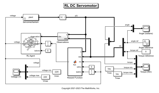

Create Model Predictive Controller

Create the open-loop dynamic model of the motor, defined in plant and the maximum admissible torque tau using a helper function.

[plant,tau] = mpcmotormodel;

Specify input and output signal types for the MPC controller. The shaft angular position is measured as first output. The second output, torque, is unmeasurable.

plant = setmpcsignals(plant, MV=1, MO=1, UO=2);

Specify constraints on the manipulated variable, and define a scale factor.

MV = struct(Min=-220, Max=220, ScaleFactor=440);

Impose torque constraints during the first three prediction steps, and specify scale factor for both shaft position and torque.

OV = struct(Min={-Inf, [-tau;-tau;-tau;-Inf]}, ...
            Max={Inf, [tau;tau;tau;Inf]}, ...
            ScaleFactor={2*pi, 2*tau});

Specify weights for the quadratic cost function to achieve angular position tracking. Set to zero the weight for the torque, thereby allowing it to float within its constraint.

Weights = struct(MV=0, MVRate=0.1, OV=[0.1 0]);

Create an MPC controller for the plant model with a sample time of 0.1 s, a prediction horizon 10 steps, and a control horizon of 2 steps, using the previously defined structures for the weights, manipulated variables, and output variables.

mpcobj = mpc(plant, 0.1, 10, 2, Weights, MV, OV);

Display the controller specifications.

mpcobj

 
MPC object (created on 05-Sep-2024 15:03:46):
---------------------------------------------
Sampling time:      0.1 (seconds)
Prediction Horizon: 10
Control Horizon:    2

Plant Model:        
                                      --------------
      1  manipulated variable(s)   -->|  4 states  |
                                      |            |-->  1 measured output(s)
      0  measured disturbance(s)   -->|  1 inputs  |
                                      |            |-->  1 unmeasured output(s)
      0  unmeasured disturbance(s) -->|  2 outputs |
                                      --------------
Indices:
  (input vector)    Manipulated variables: [1 ]
  (output vector)        Measured outputs: [1 ]
                       Unmeasured outputs: [2 ]

Disturbance and Noise Models:
        Output disturbance model: default (type "getoutdist(mpcobj)" for details)
         Measurement noise model: default (unity gain after scaling)

Weights:
        ManipulatedVariables: 0
    ManipulatedVariablesRate: 0.1000
             OutputVariables: [0.1000 0]
                         ECR: 10000

State Estimation:  Default Kalman Filter (type "getEstimator(mpcobj)" for details)

Constraints:
 -220 <= MV1 (V) <= 220, MV1/rate (V) is unconstrained,       MO1 (rad) is unconstrained
                                                        -78.54 <= UO1 (Nm)(t+1) <= 78.54
                                                        -78.54 <= UO1 (Nm)(t+2) <= 78.54
                                                        -78.54 <= UO1 (Nm)(t+3) <= 78.54
                                                          UO1 (Nm)(t+4) is unconstrained

Use built-in "active-set" QP solver with MaxIterations of 120.

The controller operates on a plant with 4 states, 1 input (voltage) and 2 output signals (angle and torque) and has the following specifications:

The cost function weights for the manipulated variable, manipulated variable rate and output variables are 0, 0.1 and [0.1 0] respectively.
The manipulated variable is constrained between -220V and 220V.
The manipulated variable rate is unconstrained.
The first output variable (angle) is unconstrained but the second (torque) is constrained between -78.54 Nm and 78.54 Nm in the first three prediction time steps and unconstrained in the fourth step.

Note that for reinforcement learning only the constraints specification from the first prediction time step will be used since the reward is computed for a single time step.

Generate the Reward Function

Generate the reward function code from specifications in the mpc object using generateRewardFunction. The code is displayed in the MATLAB Editor.

generateRewardFunction(mpcobj)

The generated reward function is a starting point for reward design. You can modify the function with different penalty function choices and tune the weights. For this example, make the following change to the generated code:

Scale the original cost weights Qy and Qmvrate by a factor of 50 and 10 respectively.
Scale the penalty weights Wy, Wmv and Wmvrate by a factor of 1e-2, 1e-3 and 1e-3 respectively.
The default exterior penalty function method is step. Change the method to quadratic.

After you make changes, the cost and penalty specifications should be as follows:

Qy      = 50 * [0.1 0];
Qmv     = 0;
Qmvrate = 10 * 0.1;
Wy      = 1e-2 * [1 1];
Wmv     = 1e-3;
Wmvrate = 1e-3;
Py      = Wy      * exteriorPenalty(y,ymin,ymax,'quadratic');
Pmv     = Wmv     * exteriorPenalty(mv,mvmin,mvmax,'quadratic');
Pmvrate = Wmvrate * exteriorPenalty(mv-lastmv,mvratemin,mvratemax,'quadratic');

For this example, the modified code has been saved in the MATLAB® function file rewardFunctionMpc.m. Display the generated reward function.

type rewardFunctionMpc.m

function reward = rewardFunctionMpc(y,refy,mv,refmv,lastmv)
% REWARDFUNCTIONMPC generates rewards from MPC specifications.
%
% Description of input arguments:
%
% y : Output variable from plant at step k+1
% refy : Reference output variable at step k+1
% mv : Manipulated variable at step k
% refmv : Reference manipulated variable at step k
% lastmv : Manipulated variable at step k-1
%
% Limitations (MPC and NLMPC):
%     - Reward computed based on first step in prediction horizon.
%       Therefore, signal previewing and control horizon settings are ignored.
%     - Online cost and constraint update is not supported.
%     - Custom cost and constraint specifications are not considered.
%     - Time varying cost weights and constraints are not supported.
%     - Mixed constraint specifications are not considered (for the MPC case).

% Reinforcement Learning Toolbox
% 02-Jun-2021 16:05:41

%#codegen

%% Specifications from MPC object
% Standard linear bounds as specified in 'States', 'OutputVariables', and
% 'ManipulatedVariables' properties
ymin = [-Inf -78.5398163397448];
ymax = [Inf 78.5398163397448];
mvmin = -220;
mvmax = 220;
mvratemin = -Inf;
mvratemax = Inf;

% Scale factors as specified in 'States', 'OutputVariables', and
% 'ManipulatedVariables' properties
Sy  = [6.28318530717959 157.07963267949];
Smv = 440;

% Standard cost weights as specified in 'Weights' property
Qy      = 50 * [0.1 0];
Qmv     = 0;
Qmvrate = 10 * 0.1;

%% Compute cost
dy      = (refy(:)-y(:)) ./ Sy';
dmv     = (refmv(:)-mv(:)) ./ Smv';
dmvrate = (mv(:)-lastmv(:)) ./ Smv';
Jy      = dy'      * diag(Qy.^2)      * dy;
Jmv     = dmv'     * diag(Qmv.^2)     * dmv;
Jmvrate = dmvrate' * diag(Qmvrate.^2) * dmvrate;
Cost    = Jy + Jmv + Jmvrate;

%% Penalty function weight (specify nonnegative)
Wy = 1e-2 * [1 1];
Wmv = 1e-3;
Wmvrate = 1e-3;

%% Compute penalty
% Penalty is computed for violation of linear bound constraints.
%
% To compute exterior bound penalty, use the exteriorPenalty function and
% specify the penalty method as 'step' or 'quadratic'.
%
% Alternatively, use the hyperbolicPenalty or barrierPenalty function for
% computing hyperbolic and barrier penalties.
%
% For more information, see help for these functions.
%
% Set Pmv value to 0 if the RL agent action specification has
% appropriate 'LowerLimit' and 'UpperLimit' values.
Py      = Wy      * exteriorPenalty(y,ymin,ymax,'quadratic');
Pmv     = Wmv     * exteriorPenalty(mv,mvmin,mvmax,'quadratic');
Pmvrate = Wmvrate * exteriorPenalty(mv-lastmv,mvratemin,mvratemax,'quadratic');
Penalty = Py + Pmv + Pmvrate;

%% Compute reward
reward = -(Cost + Penalty);
end

To integrate this reward function, open the MATLAB Function block in the Simulink model.

open_system("rl_motor/Reward Function")

Append the function with the following line of code and save the model.

r = rewardFunctionMpc(y,refy,mv,refmv,lastmv);

The MATLAB Function block will now execute rewardFunctionMpc.m during simulation.

For this example, the MATLAB Function block has already been modified and saved.

Create a Reinforcement Learning Environment

The environment dynamics are modeled in the Servomechanism subsystem. For this environment,

The observations are the reference signals (angle and torque), output variables (angle and torque), and their integrals from the last 3 time steps. The angle and torque signals are normalized by multiplying with the gain [0.1 1/tau].
The action is the voltage $V$ applied to the servomotor. The action values are limited between -220 and 220.
The sample time is $T_{s} = 0.1 s$ .
The total simulation time is $T_{f} = 20 s$ .

Specify the total simulation time and sample time.

Tf = 20;
Ts = 0.1;

Create observation and action specifications for the environment.

numObs = 24;
numAct = 1;
oinfo = rlNumericSpec([numObs 1]);
ainfo = rlNumericSpec([numAct 1], ...
    LowerLimit=-220, ...
    UpperLimit=220);

Create the reinforcement learning environment using the rlSimulinkEnv function.

blk = "rl_motor/RL Agent";
env = rlSimulinkEnv(mdl, blk, oinfo, ainfo);

Create a Reinforcement Learning Agent

The agent used in this example is a twin-delayed deep deterministic policy gradient (TD3) agent. TD3 agents use two parametrized Q-value function approximators to estimate the value (that is the expected cumulative long-term reward) of the policy. To model the parametrized Q-value function within both critics, use a neural network with two inputs (the observation and action) and one output (the value of the policy when taking a given action from the state corresponding to a given observation). For more information on TD3 agents, see Twin-Delayed Deep Deterministic (TD3) Policy Gradient Agent.

Fix the random stream for reproducibility.

rng(0,"twister");

Define each network path as an array of layer objects. Assign names to the input and output layers of each path. These names allow you to connect the paths and then later explicitly associate the network input and output layers with the appropriate environment channel.

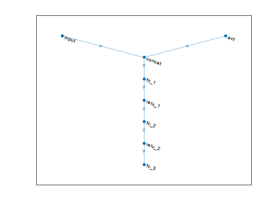
% Define paths.
mainPath = [
    featureInputLayer(numObs)
    concatenationLayer(1, 2, Name="concat")
    fullyConnectedLayer(128)
    reluLayer
    fullyConnectedLayer(64)
    reluLayer
    fullyConnectedLayer(1)
    ];
actionPath = [
    featureInputLayer(numAct, Name="act")
    ];

% Create dlnetwork object and add layers.
criticNet = dlnetwork;
criticNet = addLayers(criticNet, mainPath);
criticNet = addLayers(criticNet, actionPath);

% Connect Layers.
criticNet = connectLayers(criticNet, "act", "concat/in2");

Plot the critic network structure.

plot(criticNet);

Figure contains an axes object. The axes object contains an object of type graphplot.

Create the critic function objects using rlQValueFunction. The critic function object encapsulates the critic by wrapping around the critic deep neural network. To make sure the critics have different initial weights, explicitly initialize each network before using them to create the critics.

% Create the two critic functions for the TD3 agent
critic1 = rlQValueFunction(initialize(criticNet), oinfo, ainfo);
critic2 = rlQValueFunction(initialize(criticNet), oinfo, ainfo);

TD3 agents learn a parametrized deterministic policy over continuous action spaces, which is learned by a continuous deterministic actor. This actor takes the current observation as input and returns as output an action that is a deterministic function of the observation.

To model the parametrized policy within the actor, use a neural network with one input layer (which receives the content of the environment observation channel, as specified by obsInfo) and one output layer (which returns the action to the environment action channel, as specified by ainfo).

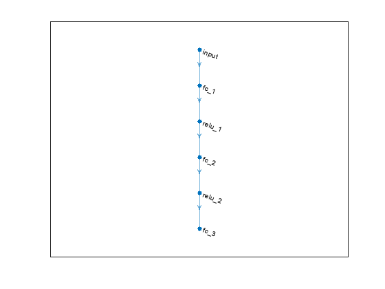
Define the network as an array of layer objects.

actorNet = [
    featureInputLayer(numObs)
    fullyConnectedLayer(128)
    reluLayer
    fullyConnectedLayer(64)
    reluLayer
    fullyConnectedLayer(numAct)
    ];

Convert to dlnetwork object.

actorNet = dlnetwork(actorNet);

Plot the actor network.

plot(actorNet);

Figure contains an axes object. The axes object contains an object of type graphplot.

Create a deterministic actor function that is responsible for modeling the policy of the agent. For more information, see rlContinuousDeterministicActor.

actor = rlContinuousDeterministicActor(actorNet, oinfo, ainfo);

Specify the following agent options using rlTD3AgentOptions:

Specify the discount factor of 0.995 to favor long-term rewards.
Store experiences in an experience buffer of maximum capacity 1e6.
Specify a mini-batch size of 1024 for learning. Smaller mini-batches are computationally efficient but may introduce variance in training. Contrarily, larger batch sizes can make the training stable but require higher memory.
Collect experiences up to 1024 steps (use the NumWarmStartSteps option) before first executing the learning algorithm.
Update the actor and critic networks using 10 learning epochs.
Specify the actor and critic learning rates to be 2e-3 and 5e-3 respectively. A large learning rate causes drastic updates which may lead to divergent behaviors, while a low value may require many updates before reaching the optimal point.
Use a gradient threshold of 1 to clip the gradients. Clipping the gradients can improve training stability.

agentOpts = rlTD3AgentOptions(SampleTime=Ts, ...
    DiscountFactor=0.995, ...
    ExperienceBufferLength=1e6, ...
    NumWarmStartSteps=1024, ...
    NumEpoch=10, ...
    MiniBatchSize=1024);

% Critic optimizer options
for idx = 1:2
    agentOpts.CriticOptimizerOptions(idx).LearnRate = 5e-3;
    agentOpts.CriticOptimizerOptions(idx).GradientThreshold = 1;
end

% Actor optimizer options
agentOpts.ActorOptimizerOptions.LearnRate = 2e-3;
agentOpts.ActorOptimizerOptions.GradientThreshold = 1;

During training, the agent explores the action space using a Gaussian action noise model. Set the standard deviation and decay rate of the noise using the ExplorationModel property. The noise has an initial standard deviation of 50 which exponentially decays at the rate of 1e-4 until it reaches a minimum value of 10. This favors exploration towards the beginning of training and exploitation in later stages.

agentOpts.ExplorationModel.StandardDeviation = 50;
agentOpts.ExplorationModel.StandardDeviationMin = 10;
agentOpts.ExplorationModel.StandardDeviationDecayRate = 1e-4;

Create the TD3 agent using the actor and critic representations. For more information on TD3 agents, see rlTD3Agent.

agent = rlTD3Agent(actor, [critic1,critic2], agentOpts);

Train the Agent

To train the agent, first specify the training options using rlTrainingOptions. For this example, use the following options:

Run each training for at most 5000 episodes, with each episode lasting at most ceil(Tf/Ts) time steps.
Stop the training when the statistic returned by the evaluator object used with train equals or exceeds the specified value of -12. At this point, the agent can track the reference signal.

trainOpts = rlTrainingOptions(...
    MaxEpisodes=5000, ...
    MaxStepsPerEpisode=ceil(Tf/Ts), ...
    StopTrainingCriteria="EvaluationStatistic", ...
    StopTrainingValue=-12, ...
    ScoreAveragingWindowLength=20);

To evaluate the agent during training, create an rlEvaluator object. Configure the evaluator to run 1 evaluation episode every 50 training episodes.

evl = rlEvaluator( ...
    NumEpisodes=1, ...
    EvaluationFrequency=50);

Fix the random stream for reproducibility.

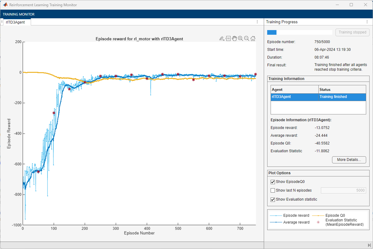
rng(0,"twister");

Train the agent using the train function. Training this agent is a computationally intensive process that may take several minutes to complete. To save time while running this example, load a pretrained agent by setting doTraining to false. To train the agent yourself, set doTraining to true.

doTraining = false;
if doTraining
    trainResult = train(agent, env, trainOpts, Evaluator=evl);
else
    load('rlDCServomotorTD3Agent.mat')
end

A snapshot of the training progress is shown in the following figure. You can expect different results due to inherent randomness in the training process.

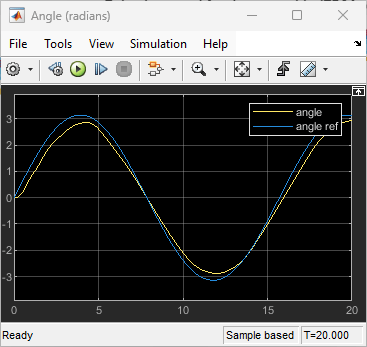
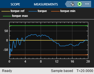
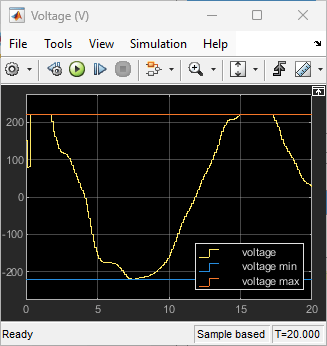
Validate Controller Response

Fix the random stream for reproducibility.

rng(0,"twister");

To validate the performance of the trained agent, simulate the model and view the response in the Scope blocks. The reinforcement learning agent is able to track the reference angle while satisfying the constraints on torque and voltage.