Train DDPG Agent to Swing Up and Balance Pendulum with Bus Signal

Pendulum Swing-Up Model with Bus

The starting model for this example is a simple frictionless pendulum. The training goal is to make the pendulum stand upright without falling over using minimal control effort.

Open the model.

mdl = "rlSimplePendulumModelBus";
open_system(mdl)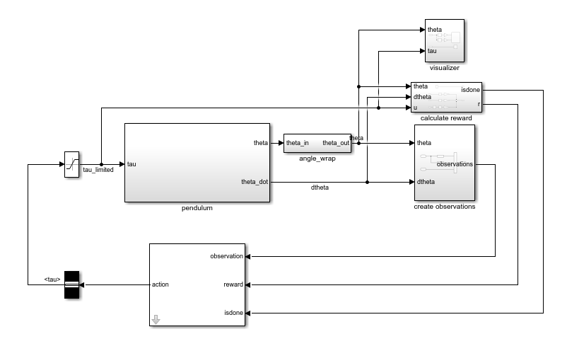

For this model:

Here:

The model used in this example is similar to the simple pendulum model described in Load Predefined Control System Environments. The difference is that the model in this example uses Simulink buses for the action and observation signals.

Create Environment Interface with Bus

The environment interface from a Simulink model is created using rlSimulinkEnv, which requires the name of the Simulink model, the path to the agent block, and observation and action reinforcement learning data specifications. For models that use bus signals for actions or observations, you can create the corresponding specifications using the bus2RLSpec function.

Specify the path to the agent block.

agentBlk = "rlSimplePendulumModelBus/RL Agent";

Create the observation Bus object. The channel names must correspond to the signal names specified in the Simulink buses used to create the observation and action signals.

obsBus = Simulink.Bus();
obs(1) = Simulink.BusElement;
obs(1).Name = "sin_theta";
obs(2) = Simulink.BusElement;
obs(2).Name = "cos_theta";
obs(3) = Simulink.BusElement;
obs(3).Name = "dtheta";
obsBus.Elements = obs;

Create the action Bus object.

actBus = Simulink.Bus();
act(1) = Simulink.BusElement;
act(1).Name = "tau";
act(1).Min = -2;
act(1).Max = 2;
actBus.Elements = act;

Create the action and observation specification objects using the Simulink buses.

obsInfo = bus2RLSpec("obsBus","Model",mdl)
actInfo = bus2RLSpec("actBus","Model",mdl)

actInfo = 
  rlNumericSpec with properties:

     LowerLimit: -2
     UpperLimit: 2
           Name: "tau"
    Description: ""
      Dimension: [1 1]
       DataType: "double"

Create the reinforcement learning environment for the pendulum model.

env = rlSimulinkEnv(mdl,agentBlk,obsInfo,actInfo);

To define the initial condition of the pendulum as hanging downward, specify an environment reset function using an anonymous function handle. This reset function sets the model workspace variable theta0 to pi.

env.ResetFcn = @(in)setVariable(in,"theta0",pi,"Workspace",mdl);

Specify the simulation time Tf and the agent sample time Ts in seconds.

Ts = 0.05;
Tf = 20;

Fix the random generator seed for reproducibility.

rng(0)

Create DDPG Agent

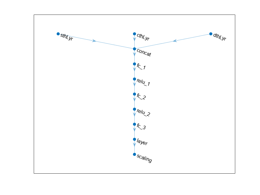
DDPG agents use a parametrized deterministic policy over continuous action spaces, which is learned by a continuous deterministic actor. This actor takes the current observation as input and returns as output an action that is a deterministic function of the observation.

To model the parametrized policy within the actor, use a neural network with three input layers (each receiving one scalar observation, as specified by obsInfo) and one output layer (which returns the action to the environment action channel, as specified by actInfo).

Define the network as an array of layer objects, and combine the outputs from the input layes using a concatenationLayer. Since the output of tanhLayer is limited between -1 and 1, scale the network output to the range of the action using scalingLayer.

For more information on creating actors based on deep neural networks, see Create Policies and Value Functions.

% Define input layers.
sinThetaInputLayer = featureInputLayer(1,Name="sthLyr");
cosThetaInputLayer = featureInputLayer(1,Name="cthLyr");
dThetaInputLayer   = featureInputLayer(1,Name="dthLyr");

% Define common path.
commonPath = [
    concatenationLayer(1,3,Name="concat")
    fullyConnectedLayer(400)
    reluLayer
    fullyConnectedLayer(300)
    reluLayer
    fullyConnectedLayer(1)
    tanhLayer
    scalingLayer(Scale=max(actInfo.UpperLimit))
    ];

Create dlnetwork object and add layers.

actorNetwork = dlnetwork;
actorNetwork = addLayers(actorNetwork,sinThetaInputLayer);
actorNetwork = addLayers(actorNetwork,cosThetaInputLayer);
actorNetwork = addLayers(actorNetwork,dThetaInputLayer);
actorNetwork = addLayers(actorNetwork,commonPath);

Connect layers.

actorNetwork = connectLayers(actorNetwork,"sthLyr","concat/in1");
actorNetwork = connectLayers(actorNetwork,"cthLyr","concat/in2");
actorNetwork = connectLayers(actorNetwork,"dthLyr","concat/in3");

Initialize network and display the number of weights.

actorNetwork = initialize(actorNetwork);
summary(actorNetwork)

   Initialized: true

   Number of learnables: 122.2k

   Inputs:
      1   'sthLyr'   1 features
      2   'cthLyr'   1 features
      3   'dthLyr'   1 features

View the actor network configuration.

plot(actorNetwork)

Create the actor using the specified deep neural network. Specify the action and observation info for the actor, as well as the names of the network input layers to be connected with the observation channels. For more information, see rlContinuousDeterministicActor.

actor = rlContinuousDeterministicActor(actorNetwork,obsInfo,actInfo,...
    "ObservationInputNames",["sthLyr","cthLyr","dthLyr"]);

DDPG agents use a parametrized Q-value function approximator to estimate the value of the policy. A Q-value function critic takes the current observation and an action as inputs and returns a single scalar as output (the estimated discounted cumulative long-term reward for which receives the action from the state corresponding to the current observation, and following the policy thereafter).

To model the parametrized Q-value function within the critic, use a neural network with four input layers (three for the observation channels, as specified by obsInfo, and the other for the action channel, as specified by actInfo) and one output layer (which returns the scalar value).

Define each network path as an array of layer objects, assigning names to the input and output layers of each path. Use the input layers previously defined for the actor.

% Define observation path.
obsPath = [
    concatenationLayer(1,3,Name="concat")
    fullyConnectedLayer(400)
    reluLayer
    fullyConnectedLayer(300,Name="obsPathOutLyr")
    ];

% Define action path.
actPath = [
    featureInputLayer(1,Name= "action")
    fullyConnectedLayer(300, ...
        Name="actPathOutLyr", ...
        BiasLearnRateFactor=0)
        ];

% Define common path.
commonPath = [
    additionLayer(2,Name="add")
    reluLayer
    fullyConnectedLayer(1,Name="CriticOutput")
    ];

Create dlnetwork object and add layers.

criticNetwork = dlnetwork;
criticNetwork = addLayers(criticNetwork,sinThetaInputLayer);
criticNetwork = addLayers(criticNetwork,cosThetaInputLayer);
criticNetwork = addLayers(criticNetwork,dThetaInputLayer);
criticNetwork = addLayers(criticNetwork,actPath);
criticNetwork = addLayers(criticNetwork,obsPath);
criticNetwork = addLayers(criticNetwork,commonPath);

Connect layers.

criticNetwork = connectLayers(criticNetwork,"sthLyr","concat/in1");
criticNetwork = connectLayers(criticNetwork,"cthLyr","concat/in2");
criticNetwork = connectLayers(criticNetwork,"dthLyr","concat/in3");
criticNetwork = connectLayers(criticNetwork,"obsPathOutLyr","add/in1");
criticNetwork = connectLayers(criticNetwork,"actPathOutLyr","add/in2");

Initialize network and display the number of weights.

criticNetwork = initialize(criticNetwork);
summary(criticNetwork)

   Initialized: true

   Number of learnables: 122.8k

   Inputs:
      1   'sthLyr'   1 features
      2   'cthLyr'   1 features
      3   'dthLyr'   1 features
      4   'action'   1 features

Create the critic approximator object using criticNet, the environment observation and action specifications, and the names of the network input layers to be connected with the environment observation and action channels. For more information, see rlQValueFunction.

critic = rlQValueFunction(criticNetwork, ...
    obsInfo,actInfo,...
    ObservationInputNames=["sthLyr","cthLyr","dthLyr"], ...
    ActionInputNames="action");

Specify options for the critic and actor using rlOptimizerOptions.

criticOptions = rlOptimizerOptions(LearnRate=1e-03,GradientThreshold=1);
actorOptions = rlOptimizerOptions(LearnRate=1e-03,GradientThreshold=1);

To create the DDPG agent, first specify the DDPG agent options using rlDDPGAgentOptions.

agentOpts = rlDDPGAgentOptions(...
    SampleTime=Ts,...
    CriticOptimizerOptions=criticOptions,...
    ActorOptimizerOptions=actorOptions,...
    ExperienceBufferLength=1e5,...
    DiscountFactor=0.99,...
    MiniBatchSize=128);
agentOpts.NoiseOptions.StandardDeviation = 0.6;

Then create the DDPG agent using the specified actor representation, critic representation, and agent options. For more information, see rlDDPGAgent.

agent = rlDDPGAgent(actor,critic,agentOpts);

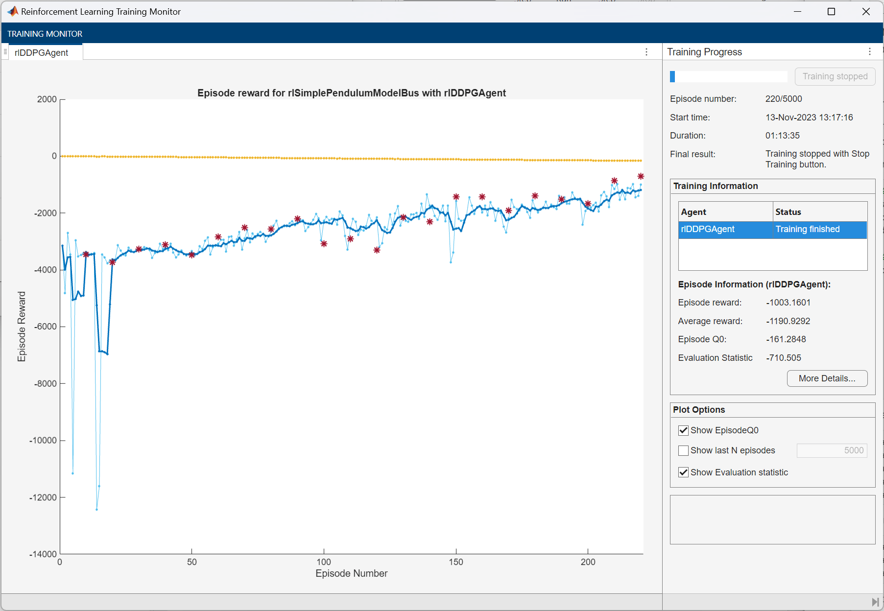
Train Agent

To train the agent, first specify the training options. For this example, use the following options:

For more information, see rlTrainingOptions.

maxepisodes = 5000;
maxsteps = ceil(Tf/Ts);
trainOpts = rlTrainingOptions(...
    MaxEpisodes=maxepisodes,...
    MaxStepsPerEpisode=maxsteps,...
    ScoreAveragingWindowLength=5,...
    Verbose=false,...
    Plots="training-progress",...
    StopTrainingCriteria="EvaluationStatistic",...
    StopTrainingValue=-740);

Train the agent using the train function. Training this agent is a computationally intensive process that takes several hours to complete. To save time while running this example, load a pretrained agent by setting doTraining to false. To train the agent yourself, set doTraining to true.

doTraining = false;
if doTraining
    % Use the rlEvaluator object to measure policy performance every 10
    % episodes
    evaluator = rlEvaluator(...
        NumEpisodes=1,...
        EvaluationFrequency=10);
    % Train the agent.
    trainingStats = train(agent,env,trainOpts,Evaluator=evaluator);
else
    % Load the pretrained agent for the example.
    load("SimulinkPendBusDDPG.mat","agent")
end

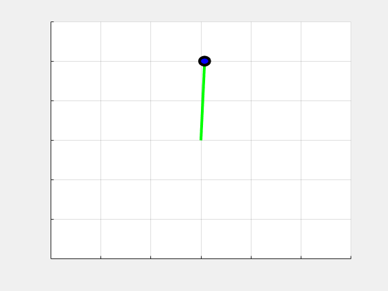
Simulate DDPG Agent

To validate the performance of the trained agent, simulate it within the pendulum environment. For more information on agent simulation, see rlSimulationOptions and sim.

simOptions = rlSimulationOptions(MaxSteps=500);
experience = sim(env,agent,simOptions);