VaR Backtesting Workflow
This example shows a value-at-risk (VaR) backtesting workflow and the use of VaR backtesting tools. For a more comprehensive example of VaR backtesting, see Value-at-Risk Estimation and Backtesting.
Step 1. Load the VaR backtesting data.
Use the VaRBacktestData.mat file to load the VaR data into the workspace. This example works with the EquityIndex, Normal95, and Normal99 numeric arrays. These arrays are equity returns and the corresponding VaR data at 95% and 99% confidence levels is produced with a normal distribution (a variance-covariance approach). See Value-at-Risk Estimation and Backtesting for an example on how to generate this VaR data.
load('VaRBacktestData')
disp([EquityIndex(1:5) Normal95(1:5) Normal99(1:5)])
-0.0043 0.0196 0.0277
-0.0036 0.0195 0.0276
-0.0000 0.0195 0.0275
0.0298 0.0194 0.0275
0.0023 0.0197 0.0278
The first column shows three losses in the first three days, but none of these losses exceeds the corresponding VaR (columns 2 and 3). The VaR model fails whenever the loss (negative of returns) exceeds the VaR.
Step 2. Create a varbacktest object.
Create a varbacktest object for the equity returns and the VaRs at 95% and 99% confidence levels.
vbt = varbacktest(EquityIndex,[Normal95 Normal99],...
   'PortfolioID','S&P', ...
   'VaRID',{'Normal95' 'Normal99'}, ...
   'VaRLevel',[0.95 0.99],'Time', Date);
disp(vbt)
  varbacktest with properties:

    PortfolioData: [1043×1 double]
          VaRData: [1043×2 double]
             Time: [1043×1 datetime]
      PortfolioID: "S&P"
            VaRID: ["Normal95"    "Normal99"]
         VaRLevel: [0.9500 0.9900]
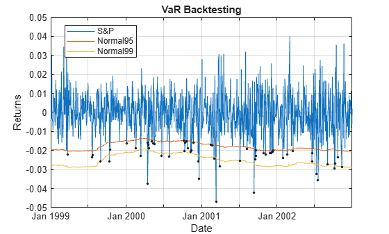
Step 3. Generate a VaR backtesting plot.
Use the plot function to visualize the VaR backtesting data. This type of visualization is a common first step when performing a VaR backtesting analysis.
plot(vbt)
ylabel("Returns")
xlabel("Date")
Step 4. Run a summary report.
Use the summary function to obtain a summary for the number of observations, the number of failures, and other simple metrics.
summary(vbt)
ans=2×10 table
    PortfolioID      VaRID       VaRLevel    ObservedLevel    Observations    Failures    Expected    Ratio     FirstFailure    Missing
    ___________    __________    ________    _____________    ____________    ________    ________    ______    ____________    _______

       "S&P"       "Normal95"      0.95         0.94535           1043           57        52.15       1.093         58            0
       "S&P"       "Normal99"      0.99          0.9837           1043           17        10.43      1.6299        173            0
Step 5. Run all tests.
Use the runtests function to display the final test results all at once.
runtests(vbt)
ans=2×11 table
    PortfolioID      VaRID       VaRLevel      TL       Bin       POF       TUFF       CC       CCI       TBF       TBFI
    ___________    __________    ________    ______    ______    ______    ______    ______    ______    ______    ______

       "S&P"       "Normal95"      0.95      green     accept    accept    accept    accept    accept    reject    reject
       "S&P"       "Normal99"      0.99      yellow    reject    accept    accept    accept    accept    accept    accept
Step 6. Run individual tests.
After running all tests, you can investigate the details of particular tests. For example, use the tl function to run the traffic light test.
tl(vbt)
ans=2×9 table
    PortfolioID      VaRID       VaRLevel      TL      Probability     TypeI     Increase    Observations    Failures
    ___________    __________    ________    ______    ___________    _______    ________    ____________    ________

       "S&P"       "Normal95"      0.95      green       0.77913      0.26396          0         1043           57
       "S&P"       "Normal99"      0.99      yellow      0.97991      0.03686    0.26582         1043           17
Step 7. Create VaR backtests for multiple portfolios.
You can create VaR backtests for different portfolios, or the same portfolio over different time windows using the select function. Run tests over two different subwindows of the original test window.
Ind1 = year(Date)<=2000;
Ind2 = year(Date)>2000;

vbt1 = select(vbt, ...
    'TimeRange', Ind1, ...
    'NewPortfolioID', 'S&P, 1999-2000');

vbt2 = select(vbt, ...
    'TimeRange', Ind2, ...
    'NewPortfolioID', 'S&P, 2001-2002');
Step 8. Display a summary report for both portfolios.
Use the summary function to display a summary for both portfolios.
Summary = [summary(vbt1); summary(vbt2)];
disp(Summary)
      PortfolioID         VaRID       VaRLevel    ObservedLevel    Observations    Failures    Expected    Ratio     FirstFailure    Missing
    ________________    __________    ________    _____________    ____________    ________    ________    ______    ____________    _______

    "S&P, 1999-2000"    "Normal95"      0.95         0.94626           521            28        26.05      1.0749         58            0
    "S&P, 1999-2000"    "Normal99"      0.99         0.98464           521             8         5.21      1.5355        173            0
    "S&P, 2001-2002"    "Normal95"      0.95         0.94444           522            29         26.1      1.1111         35            0
    "S&P, 2001-2002"    "Normal99"      0.99         0.98276           522             9         5.22      1.7241         45            0
Step 9. Run all tests for both portfolios.
Use the runtests function to display the final test result for both portfolios.
Results = [runtests(vbt1);runtests(vbt2)];
disp(Results)
      PortfolioID         VaRID       VaRLevel      TL       Bin       POF       TUFF       CC       CCI       TBF       TBFI
    ________________    __________    ________    ______    ______    ______    ______    ______    ______    ______    ______

    "S&P, 1999-2000"    "Normal95"      0.95      green     accept    accept    accept    accept    accept    reject    reject
    "S&P, 1999-2000"    "Normal99"      0.99      green     accept    accept    accept    accept    accept    accept    accept
    "S&P, 2001-2002"    "Normal95"      0.95      green     accept    accept    accept    accept    accept    accept    accept
    "S&P, 2001-2002"    "Normal99"      0.99      yellow    accept    accept    accept    accept    accept    accept    accept
Step 10. List exceptions.
Use the exceptions function to list all the exceptions in the full test window. An exception is a data point where -portfolioValue > threshold*varValue, a loss is defined as -portfolioValue for a given point in time, and the SeverityRatio is the ratio Loss/VaR.
exceptionsTable = exceptions(vbt);
head(exceptionsTable)
       Time          Loss      Normal95    SeverityRatio
    ___________    ________    ________    _____________

    23-Mar-1999    0.022232    0.020108       1.1057
    20-Jul-1999    0.023592     0.01998       1.1808
    22-Jul-1999    0.022426    0.019963       1.1234
    31-Aug-1999     0.02561    0.017744       1.4433
    13-Oct-1999    0.025715    0.015562       1.6525
    15-Oct-1999    0.019577    0.015711       1.2461
    04-Jan-2000    0.016179    0.014776       1.0949
    18-Feb-2000    0.018806    0.014471       1.2996
See Also
varbacktest | tl | bin | pof | tuff | cc | cci | tbf | tbfi | summary | runtests | select | plot | exceptions | append