Four-Wheel Ground Following

R2026b

Compute terrain-aligned 3-D pose for four-wheeled vehicle

Since R2026b

Libraries:
Offroad Autonomy Library / Ground Following

Description

Add-On Required: This feature requires the Robotics System Toolbox Offroad Autonomy Library add-on.

The Four-Wheel Ground Following block computes a terrain-aligned 3-D pose (translation and rotation) for a four-wheeled vehicle moving over uneven ground in Simulink^®, without requiring Unreal Engine^® visualization. The block uses the 2-D pose of the rear-axle frame of the vehicle chassis and the wheel parameters to determine the vehicle translation and orientation where the wheels remain in contact with the terrain surface. The output pose represents the vehicle chassis aligned with the terrain geometry.

The chassis is modeled as a rectangular frame whose length and width are equal to the wheel base and track width respectively, and the rear-axle frame is placed at the midpoint of the rear axle of this rectangular chassis frame. All input and output poses use a right-handed coordinate system. The block uses meters for all distance values and meters per pixel for resolution.

Use this block for kinematic simulation of wheeled vehicles where you need ground following, but do not need to account for wheel dynamics or suspension modeling. You can use the outputs with the Chassis To Tree-Frame Motion block to simulate (Inertial Measurement Unit) IMU readings at sensor mounting locations defined on a rigid body tree.

Ground Elevation Lookup

The Four-Wheel Ground Following block gathers the elevation values of the wheels by projecting XY-plane of the wheel frame, which is always vertically downwards in the world frame. It then uses the coordinates of the projection to look up the terrain elevation from the heightmap using bilinear interpolation. In contrast, the Simulation 3D Four-Wheel Ground Following block, uses ray tracing perpendicular to the chassis in an Unreal Engine scene.

This figure illustrates the difference between the Simulink vertical projection approach and the Unreal^® perpendicular ray tracing approach.

This distinction means:

On flat or gently sloped terrain, results closely match the Simulation 3D Four-Wheel Ground Following block.
On steep terrain, the vertical projection may yield different contact points than the chassis-perpendicular projection used in Unreal Engine.

Comparison with Simulation 3D Ground-Following Block

This table summarizes the differences between the Four-Wheel Ground Following block and the Simulation 3D Four-Wheel Ground Following block.

Aspect	Four-Wheel Ground Following	Simulation 3D Four-Wheel Ground Following
Requires Unreal Engine	No	Yes
Terrain source	16-bit grayscale PNG heightmap	Unreal Engine scene
Ray projection	Vertical (world-frame Z-down)	Perpendicular to chassis
Output match	Not an exact match with the Simulation 3D Four-Wheel Ground Following block	Native Unreal Engine output

Examples

expand all

Simulate Ground Following and Visualize Robot on Terrain

Open Live Script

This example demonstrates how to simulate a four-wheeled robot following terrain using the Four-Wheel Ground Following block in Simulink®, without requiring Unreal Engine or any other 3-D simulation environment.

The example workflow consists of:

Generating a terrain heightmap from peaks function
Deriving chassis parameters from a rigidBodyTree object
Configuring and running the Four-Wheel Ground Following block
Interpreting the block outputs
Simulating the robot on the terrain surface

Generate Terrain Heightmap

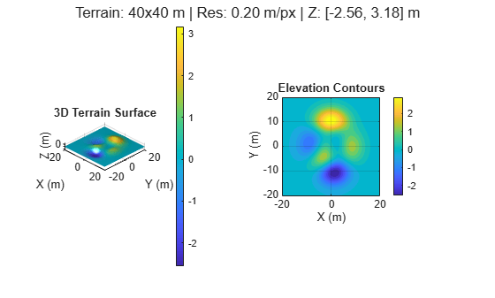
The helper script generateTerrainHeightmap creates a smoothed peaks-based terrain and encodes it as a 16-bit PNG heightmap. The heightmap uses the Unreal Engine encoding convention where pixel value 32768 corresponds to zero elevation:

pixel = Z x (128/zScale) + 32768

The script produces a workspace variable terrainMeta containing the heightmap file path, resolution, terrain size, origin, and elevation scale, all of which are used to configure the block.

generateTerrainHeightmap

Terrain generated:
  Grid size:    201 x 201 pixels
  World extent: 40 x 40 m
  Resolution:   0.20 m/pixel
  Origin:       [-20.0, -20.0, 0.0] m
  Z range:      [-2.56, 3.18] m
  Heightmap saved: C:\Users\user\OneDrive - MathWorks\Documents\MATLAB\ExampleManager\user.Bdoc26b.j3322667\offroad_autonomy-ex81148826\terrain_heightmap.png

Figure Generated Terrain contains 2 axes objects and another object of type subplottext. Axes object 1 with title 3D Terrain Surface, xlabel X (m), ylabel Y (m) contains an object of type surface. Axes object 2 with title Elevation Contours, xlabel X (m), ylabel Y (m) contains an object of type contour.

Extract Chassis Parameters from Robot Model

The helper script extractChassisParams loads the Clearpath Husky rigid body tree model and derives the wheel layout directly from the model transforms and collision geometry. This produces a robot struct used by the block.

You can derive these parameters from any rigidBodyTree object or URDF:

extractChassisParams

Robot: Clearpath Husky
  WheelBase:    0.5120 m
  TrackWidth:   0.5708 m
  WheelRadius:  0.1651 m
  RearAxlePose: T = [-0.2560, 0.0000, 0.0328] m

Chassis Parameters (derived from rigidBodyTree):
  WheelBase:    0.5120 m (front-to-rear axle distance)
  TrackWidth:   0.5708 m (left-to-right wheel distance)
  WheelRadius:  0.1651 m (from collision cylinder)
  RearAxlePose: translation = [-0.2560, 0.0000, 0.0328] m

disp("  WheelBase:   " + robot.wheelBase + " m")

  WheelBase:   0.512 m

disp("  TrackWidth:  " + robot.trackWidth + " m")

  TrackWidth:  0.5708 m

disp("  WheelRadius: " + robot.wheelRadius + " m")

  WheelRadius: 0.1651 m

disp("  RearAxlePose:   translation = [" ...
    + robot.rearAxlePose(1,4) + ", " ...
    + robot.rearAxlePose(2,4) + ", " ...
    + robot.rearAxlePose(3,4) + "] m")

  RearAxlePose:   translation = [-0.256, 0, 0.03282] m

Open Simulink Model

The model groundFollowingModel contains four key blocks:

Constant block (2.0 m/s) — Forward velocity input
Sine Wave block (0.5 amplitude, 0.15 Hz) — Steering rate oscillation
Ackermann Kinematic Model — Computes 2D planar pose (X, Y, Yaw)
Four-Wheel Ground Following — Projects the planar pose onto the 3-D terrain surface

open_system("groundFollowingModel");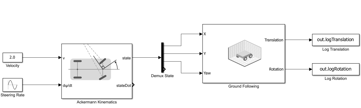

Configure Block Parameters

The Four-Wheel Ground Following block mask parameters reference workspace variables set by the helper scripts:

Block Parameter	Workspace Variable	Description
Wheelbase (m)	`robot.wheelBase`	Front-to-rear axle distance
Track width (m)	`robot.trackWidth`	Left-to-right wheel distance
Elevation scale (m/pixel)	`terrainMeta.zScale`	Maps pixel values to meters
Wheel radius (m)	`robot.wheelRadius`	Wheel radius from collision geometry
Rear axle pose	`robot.rearAxlePose`	4x4 transform from `base_link` to rear-axle frame
Resolution (m/pixel)	`terrainMeta.resolution * [1 1]`	Pixel spacing in X and Y
Origin (m)	`terrainMeta.origin`	World position of terrain grid start
File path	`terrainMeta.heightmapFile`	Path to 16-bit PNG

Inputs: X, Y, and Yaw of the rear axle frame in the world frame (from Ackermann kinematic model).

Outputs: Translation (1x3 vector in meters) and Rotation (3x3 rotation matrix) of the vehicle origin frame, base_link, on the terrain. The block internally applies wheel radius to lift above the contact plane and rear axle pose to transform from the rear-axle frame to the vehicle origin.

Run Simulation

Simulate the model. The Ackermann Kinematic Model drives the vehicle at constant speed with oscillating steering, while the Four-Wheel Ground Following block computes the terrain-following pose at each timestep.

out = sim("groundFollowingModel.slx");
logTranslation = out.logTranslation;
logRotation = out.logRotation;

Interpret Block Outputs

The block outputs the vehicle origin frame (base_link), which accounts for wheel radius and rear axle pose internally. Extract position and Euler angles from the logged data.

time = logTranslation.Time;
nSteps = length(time);
pos = squeeze(logTranslation.Data);
if size(pos, 2) ~= 3
    pos = pos';
end
roll = zeros(nSteps, 1);
pitch = zeros(nSteps, 1);
yaw = zeros(nSteps, 1);
rotData = squeeze(logRotation.Data);
for k = 1:nSteps
    if ndims(rotData) == 3
        R = rotData(:,:,k);
    else
        R = reshape(rotData(k,:), 3, 3)';
    end
    pitch(k) = asin(-R(3,1));
    roll(k) = atan2(R(3,2), R(3,3));
    yaw(k) = atan2(R(2,1), R(1,1));
end

Visualize Block Outputs

Elevation Profile

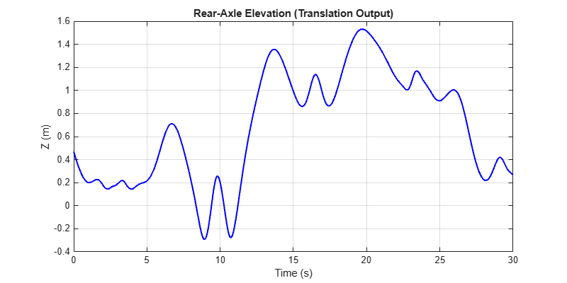
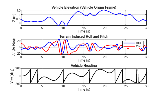
The Translation output Z component shows how the vehicle origin (base_link) follows the terrain elevation along its driven path..

figure("Position", [100, 100, 800, 400]);
plot(time, pos(:,3), "b-", "LineWidth", 1.5);
xlabel("Time (s)"); ylabel("Z (m)");
title("Rear-Axle Elevation (Translation Output)");

Figure contains an axes object. The axes object with title Rear-Axle Elevation (Translation Output), xlabel Time (s), ylabel Z (m) contains an object of type line.

grid on;

Roll and Pitch

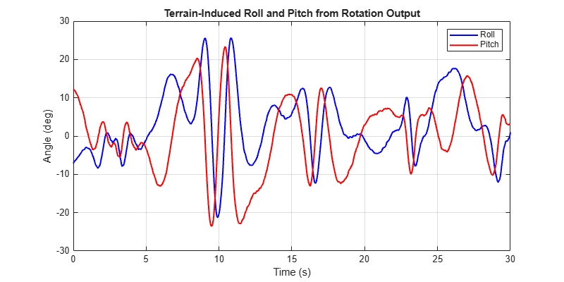
The Rotation output encodes terrain-induced body tilts. Roll and pitch arise from the ground plane fit through the four wheel contact points, not from physics simulation.

figure("Position", [100, 100, 800, 400]);
plot(time, rad2deg(roll), "b-", time, rad2deg(pitch), "r-", "LineWidth", 1.5);
xlabel("Time (s)"); ylabel("Angle (deg)");
title("Terrain-Induced Roll and Pitch from Rotation Output");
legend("Roll", "Pitch");
grid on;

Figure contains an axes object. The axes object with title Terrain-Induced Roll and Pitch from Rotation Output, xlabel Time (s), ylabel Angle (deg) contains 2 objects of type line. These objects represent Roll, Pitch.

Vehicle Heading

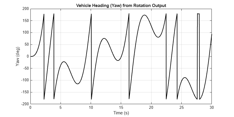
The yaw component of the Rotation output tracks the vehicle heading, driven by the Ackermann steering input.

figure("Position", [100, 100, 800, 400]);
plot(time, rad2deg(yaw), "k-", "LineWidth", 1.5);
xlabel("Time (s)"); ylabel("Yaw (deg)");
title("Vehicle Heading (Yaw) from Rotation Output"); grid on;

Figure contains an axes object. The axes object with title Vehicle Heading (Yaw) from Rotation Output, xlabel Time (s), ylabel Yaw (deg) contains an object of type line.

Review Simulation Results

totalDist = sum(sqrt(diff(pos(:,1)).^2 + diff(pos(:,2)).^2));
disp("Simulation Results:")

Simulation Results:

disp("  Duration:  " + time(end) + " s")

  Duration:  30 s

disp("  Distance:  " + totalDist + " m")

  Distance:  62.1547 m

disp("  Max roll:  " + max(abs(rad2deg(roll))) + " deg")

  Max roll:  25.582 deg

disp("  Max pitch: " + max(abs(rad2deg(pitch))) + " deg")

  Max pitch: 23.542 deg

disp("  Z range:   [" + min(pos(:,3)) + ", " + max(pos(:,3)) + "] m")

  Z range:   [-0.29073, 1.5317] m

Simulate Robot on Terrain

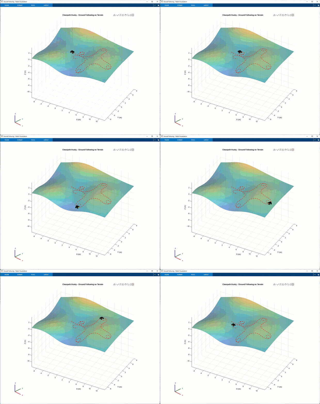
The helper script visualizeGroundFollowing builds a floating-base rigid body tree and animates the Husky traversing the terrain surface. It uses the block outputs (Translation and Rotation) directly to place the robot mesh.

visualizeGroundFollowing

Simulation Results:
  Duration:   30.0 s
  Distance:   62.2 m
  Max roll:   25.58 deg
  Max pitch:  23.54 deg
  Z range:    [-0.29, 1.53] m

Ground-following simulation of Clearpath Husky robot using Four-Wheel Ground Following block in Simulink.

Limitations

This block does not model wheel dynamics, suspension, or tire deformation. It computes a purely kinematic terrain-following pose.
The Resolution (m / pixel) parameter requires a two-element vector. Uniform resolution must be specified as [res, res].

Ports

Input

expand all

X — x-coordinate of rear-axle frame in right-handed world frame
scalar

x-coordinate of the rear-axle frame in the right-handed world frame, specified as a numeric scalar, in meters.

Data Types: double

Y — y-coordinate of rear-axle frame in right-handed world frame
scalar

y-coordinate of the rear-axle frame in the right-handed world frame, specified as a numeric scalar, in meters.

Data Types: double

Yaw — Yaw angle of rear-axle frame in right-handed world frame
scalar

Yaw angle of the rear-axle frame in the right-handed world frame, specified as a numeric scalar, in radians.

Data Types: double

Output

expand all

Translation — Translation of rear-axle frame in right-handed world frame
vector

Translation of the rear-axle frame in the right-handed world frame, returned as a 1-by-3 row vector of the form [x y z], in meters. The z-component represents the mean elevation of the rear-axle contact points on the terrain.

Data Types: double

Rotation — Rotation of rear-axle frame in right-handed world frame
vector

Rotation of the rear-axle frame in the right-handed world frame, returned as a 1-by-3 row vector of rotation matrix in the ZYX sequence (yaw, pitch, roll), in radians. The pitch and roll components are computed from terrain contact elevations at the four wheel positions.

Data Types: double

Parameters

expand all

Chassis

Track width (m) — Distance between left and right wheels on front and rear axles
`1.0` (default) | positive scalar

Distance between the left and right wheels on the front and rear axles, specified as a positive scalar. Units in meters.

You can derive this value from a rigidBodyTree object or URDF file by computing the distance between the left and right rear wheel links:

rbt = loadrobot("clearpathHusky");
homecfg = homeConfiguration(rbt);

% Track width: distance between left and right rear wheels
trackwidth = norm(tform2trvec( ...
    getTransform(rbt, homecfg, "rear_left_wheel_link", "rear_right_wheel_link")));

Wheel base (m) — Distance between rear and front wheels on same side
`1.0` (default) | positive scalar

Distance in meters between the rear and front wheels on the same side, specified as a positive scalar.

You can derive this value from a rigidBodyTree object or URDF file by computing the distance between the rear and front wheel links on the same side:

% Wheelbase: distance between rear and front wheels on the same side
wheelbase = norm(tform2trvec( ...
    getTransform(rbt, homecfg, "rear_left_wheel_link", "front_left_wheel_link")));

Wheel radius (m) — Radius of rear wheels
`0.05` (default) | nonnegative scalar

Radius of the rear wheels, specified as a nonnegative scalar. Units in meters.

The block uses this value to offset the rear-axle frame vertically above the terrain contact point. A wheel radius of zero places the rear-axle frame origin directly on the ground plane.

Rear axle pose — Pose of rear-axle frame with respect to vehicle origin frame
`eye(4)` (default) | 4-by-4 homogeneous transformation matrix

Pose of the frame centered at the rear axle with respect to the vehicle origin frame, specified as a 4-by-4 homogeneous transformation matrix.

Use this parameter to account for the offset between the vehicle origin (for example, the base frame of a rigidBodyTree model) and the rear-axle frame. When the vehicle origin coincides with the rear-axle frame, use the default value eye(4).

Terrain

File path — Path to 16-bit grayscale PNG heightmap image representing terrain elevation
`heightmap.png` (default) | character vector | string scalar

Path to a 16-bit grayscale PNG heightmap image representing terrain elevation, specified as a character vector or string scalar. The path can be absolute or relative to the current working folder.

The heightmap does not have to come from Unreal Engine. You can obtain 16-bit grayscale PNG heightmaps from other sources such as GIS elevation data and import them into MATLAB^®.

To export a heightmap from Unreal Engine:

In the Unreal Editor, select the Landscape object and go to Landscape > Manage > Import/Export > Export.
Verify the heightmap file path, check whether the Flip Y Axis option is enabled, and click Export. The editor saves the heightmap as a 16-bit grayscale PNG file.
From the General tab of the Landscape object, copy the Location (Translation), Rotation, and Scale values. You need these values to set the Origin (m), Elevation scale (m/pixel), and Resolution (m/pixel) block parameters.
Convert all values from Unreal centimeters to MATLAB meters by dividing by 100.

Origin (m) — Offset of the heightmap origin in world frame
`[0.0, 0.0, 0.0]` (default) | three-element row vector

Offset of the heightmap origin in the world frame, specified as a three-element row vector of the form [x y z]. Units in meters.

The terrain origin is assumed to be at the center of the heightmap image. Use this parameter to offset the terrain origin to align with your world-frame coordinate system.

When importing terrain from Unreal Engine, convert the Landscape Location (Translation) values from centimeters to meters and specify them here.

Elevation scale (m/pixel) — Scale factor that converts heightmap pixel values into real-world elevation units
`1.0` (default) | positive scalar

Scale factor that converts heightmap pixel values to real-world elevation units, specified as a positive scalar. The unit for the elevation scale is meters per pixel intensity value.

When importing terrain from Unreal Engine, the heightmap decoding formula is:

Z = (raw − 32768) × (ZScale / 128),

where raw is the 16-bit pixel value and ZScale is the Unreal Landscape Z-scale converted from centimeters to meters.

Resolution (m/pixel) — Scale factor that converts pixel spacing into real-world distances
`[1.0, 1.0]` (default) | two-element row vector of positive scalars

Scale factor that converts pixel spacing into real-world distances in the x and y directions, specified as a two-element row vector of positive scalars of the form [resX resY] in meters per pixel.

When importing a terrain from Unreal Engine, compute the resolution from the Landscape X and Y scale values by converting from centimeters to meters.

Simulate using — Type of simulation to run
`Interpreted execution` (default) | `Code generation`

Specify the type of simulation to run.

Code generation — Simulate model using generated C code. The first time you run a simulation, Simulink generates C code for the block. Simulink reuses the C code for subsequent simulations, if the model is unchanged from the previous run.
Interpreted execution — Simulate model using the MATLAB interpreter. For more information, see Interpreted Execution vs. Code Generation (Simulink).

Tunable: No

More About

expand all

Coordinate Frames

The block uses the following coordinate frames:

World frame — The global reference frame in which the X, Y, and Yaw inputs and the Translation and Rotation outputs are expressed. This is a right-handed coordinate system.
Rear-axle frame — A body-fixed frame located at the midpoint of the rear axle. The Four-Wheel Ground Following block computes the 3-D pose of this frame by aligning the chassis with the terrain.
Terrain frame — A local frame whose origin is at the center of the heightmap image. The Origin (m) parameter offsets this frame in the world frame.

Units

All distances are in meters. All angles are in radians. If you import terrain data from Unreal Engine, you must convert the distance from centimeters to meters.

Tips

When importing terrain from Unreal Engine, all Unreal values are in centimeters. Divide Translation and Scale values by 100 to convert to meters before entering them as block parameters.
The terrain origin is at the center of the heightmap image. Use the Origin (m) parameter to translate the terrain to the desired location in the world frame.
You can feed the Translation and Rotation outputs of this block back into an Unreal Engine simulation to enforce an exact match between Simulink and Unreal ground-following results.
To simulate IMU readings, connect the Translation and Rotation outputs to the Chassis To Tree-Frame Motion block, which transforms velocities and accelerations to a target sensor frame on a rigid body tree.

Algorithms

expand all

The block computes the 3-D pose of the rear-axle frame by aligning it with the terrain using wheel contact elevations.

Wheel Contact Point Projection

Given the planar rear-axle pose (x, y, θ) and the chassis dimensions (track width and wheel base), the block computes the four wheel positions in the world frame. Each wheel position is projected vertically downwards (Z-down in world frame) onto the terrain heightmap. The terrain elevation at each projected point is obtained using bilinear interpolation of the heightmap data.

Mean Elevations

Given the ground elevations at the four wheel contact points [z_FL, z_FR, z_RL, z_RR], the block computes mean elevations, where FL is front-left, FR is front-right, RL is rear-left, and RR is rear-right:

Front axle — z_front = (z_FL + z_FR)/2
Rear axle — z_rear = (z_RL + z_RR)/2
Left wheels — z_left = (z_FL + z_RL)/2
Right wheels — z_right = (z_FR + z_RR)/2

Ground-Aligned Orientation

The ground-aligned orientation of the rear-axle frame is defined using yaw-pitch-roll angles, where ψ is yaw, ϕ is pitch, ρ is roll, and θ is the input yaw angle of the rear-axle frame:

Yaw — ψ = θ
Pitch (longitudinal slope) — ϕ = arctan((z_rear − z_front)/wheel base)
Roll (lateral slope) — ρ = arctan((z_left − z_right)/track width)

The 3-by-3 rotation matrix is constructed as

R = R_z(ψ) R_y(ϕ) R_x(ρ).

Translation and World Pose

The translation of the rear-axle frame in the world frame is

t = [x, y, z_rear].

The block returns the world pose of the rear-axle frame as the 4-by-4 homogeneous transformation matrix

T_world = [R, t; 0, 1],

where R is the 3-by-3 rotation matrix and t is the 3-by-1 translation vector.

The block outputs the translation t and the Euler angle decomposition [ψ, ϕ, ρ] of R as the Translation and Rotation outputs, respectively.

Version History

Introduced in R2026b

Four-Wheel Ground Following

Description

Ground Elevation Lookup

Comparison with Simulation 3D Ground-Following Block

Examples

Simulate Ground Following and Visualize Robot on Terrain

Limitations

Ports

Input

X — x-coordinate of rear-axle frame in right-handed world frame scalar

Y — y-coordinate of rear-axle frame in right-handed world frame scalar

Yaw — Yaw angle of rear-axle frame in right-handed world frame scalar

Output

Translation — Translation of rear-axle frame in right-handed world frame vector

Rotation — Rotation of rear-axle frame in right-handed world frame vector

Parameters

Chassis

Track width (m) — Distance between left and right wheels on front and rear axles 1.0 (default) | positive scalar

Wheel base (m) — Distance between rear and front wheels on same side 1.0 (default) | positive scalar

Wheel radius (m) — Radius of rear wheels 0.05 (default) | nonnegative scalar

Rear axle pose — Pose of rear-axle frame with respect to vehicle origin frame eye(4) (default) | 4-by-4 homogeneous transformation matrix

Terrain

File path — Path to 16-bit grayscale PNG heightmap image representing terrain elevation heightmap.png (default) | character vector | string scalar

Origin (m) — Offset of the heightmap origin in world frame [0.0, 0.0, 0.0] (default) | three-element row vector

Elevation scale (m/pixel) — Scale factor that converts heightmap pixel values into real-world elevation units 1.0 (default) | positive scalar

Resolution (m/pixel) — Scale factor that converts pixel spacing into real-world distances [1.0, 1.0] (default) | two-element row vector of positive scalars

Simulate using — Type of simulation to run Interpreted execution (default) | Code generation

More About

Coordinate Frames

Units

Tips

Algorithms

Wheel Contact Point Projection

Mean Elevations

Ground-Aligned Orientation

Translation and World Pose

Version History

See Also

X — x-coordinate of rear-axle frame in right-handed world frame
scalar

Y — y-coordinate of rear-axle frame in right-handed world frame
scalar

Yaw — Yaw angle of rear-axle frame in right-handed world frame
scalar

Translation — Translation of rear-axle frame in right-handed world frame
vector

Rotation — Rotation of rear-axle frame in right-handed world frame
vector

Track width (m) — Distance between left and right wheels on front and rear axles
`1.0` (default) | positive scalar

Wheel base (m) — Distance between rear and front wheels on same side
`1.0` (default) | positive scalar

Wheel radius (m) — Radius of rear wheels
`0.05` (default) | nonnegative scalar

Rear axle pose — Pose of rear-axle frame with respect to vehicle origin frame
`eye(4)` (default) | 4-by-4 homogeneous transformation matrix

File path — Path to 16-bit grayscale PNG heightmap image representing terrain elevation
`heightmap.png` (default) | character vector | string scalar

Origin (m) — Offset of the heightmap origin in world frame
`[0.0, 0.0, 0.0]` (default) | three-element row vector

Elevation scale (m/pixel) — Scale factor that converts heightmap pixel values into real-world elevation units
`1.0` (default) | positive scalar

Resolution (m/pixel) — Scale factor that converts pixel spacing into real-world distances
`[1.0, 1.0]` (default) | two-element row vector of positive scalars

Simulate using — Type of simulation to run
`Interpreted execution` (default) | `Code generation`