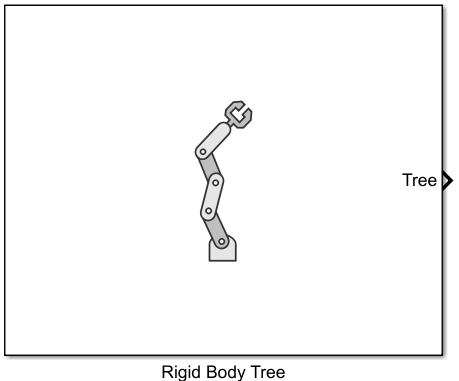
Rigid Body Tree
Libraries:
Robotics System Toolbox /
Collision Detection
Description
The Rigid Body Tree block outputs a rigid body tree robot model. A rigid body tree is a representation of the connectivity of rigid bodies with joints.
A rigid body tree model is represented in MATLAB® as a rigidBodyTree object, made up of rigid bodies
as rigidBody objects. Each rigid body has a rigidBodyJoint object associated with it that defines how it can move relative to
its parent body.
You can use the loadrobot
function to load a rigid body tree model from the Robot Library, or use the importrobot function to import robot models from Simscape™
Multibody™ models or robot model files such as URDFs.
Examples
Use the loadrobot function to load a robot model from the Robot Library and set up the collision environment.
robot = loadrobot("abbIrb120",DataFormat="row");
rad = 0.08;
len = 0.75;
pose1 = trvec2tform([0.4 -0.35 0.3]);
pose2 = trvec2tform([0 0.3 0.5]);
cylinder = collisionCylinder(rad,len,Pose=pose1);
sphere = collisionSphere(rad,Pose=pose2);
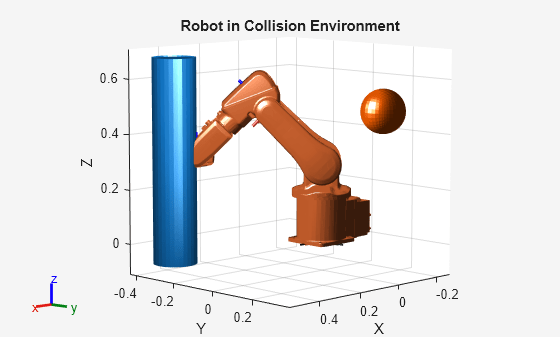
Show the robot with the collision environment. In this case, you can see the robot collides with the cylinder.
show(robot,[-pi/4 pi/4 0 0 -pi/4 0]);
hold on
showCollisionArray({cylinder,sphere});
title("Robot in Collision Environment")
hold on
open_system("RBTCheckCollisionModel");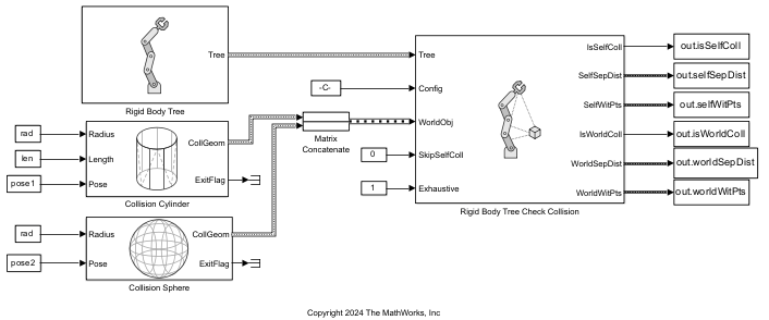
out = sim("RBTCheckCollisionModel");### Building simulation target for model: 'RBTCheckCollisionModel'.
/mathworks/devel/bat/filer/batfs2566-0/Bdoc26a.3233028/build/runnable/matlab/bin/mex -R2018a -c -DMATLAB_MEX_FILE -I"/mathworks/devel/bat/filer/batfs2566-0/Bdoc26a.3233028/build/runnable/matlab/extern/include" -I"/mathworks/devel/bat/filer/batfs2566-0/Bdoc26a.3233028/build/runnable/matlab/simulink/include" -I"/mathworks/devel/bat/filer/batfs2566-0/Bdoc26a.3233028/build/runnable/matlab/rtw/c/src" -I"/tmp/Bdoc26a_3233028_1679788/tpe812315a/robotics-ex92028207" -I"/tmp/Bdoc26a_3233028_1679788/tpe812315a/robotics-ex92028207/slprj/_cprj" -I"/tmp/Bdoc26a_3233028_1679788/tpe812315a/robotics-ex92028207/slprj/_cgxe/RBTCheckCollisionModel/src" -I"/mathworks/devel/bat/filer/batfs2566-0/Bdoc26a.3233028/build/runnable/matlab/extern/include/shared_robotics" -I"/mathworks/devel/bat/filer/batfs2566-0/Bdoc26a.3233028/build/runnable/matlab/extern/include/shared_robotics/collfcncodegen" -I"/mathworks/devel/bat/filer/batfs2566-0/Bdoc26a.3233028/build/runnable/matlab/toolbox/shared/robotics/externalDependency/libccd/src" -I"/mathworks/devel/bat/filer/batfs2566-0/Bdoc26a.3233028/build/runnable/matlab/toolbox/shared/robotics/externalDependency/libccd/src/ccd" CFLAGS="\$CFLAGS -w -Dccd_EXPORTS" RBTCheckCollisionModel_cgxe.c
Building with 'gcc'.
MEX completed successfully.
/mathworks/devel/bat/filer/batfs2566-0/Bdoc26a.3233028/build/runnable/matlab/bin/mex -R2018a -c -DMATLAB_MEX_FILE -I"/mathworks/devel/bat/filer/batfs2566-0/Bdoc26a.3233028/build/runnable/matlab/extern/include" -I"/mathworks/devel/bat/filer/batfs2566-0/Bdoc26a.3233028/build/runnable/matlab/simulink/include" -I"/mathworks/devel/bat/filer/batfs2566-0/Bdoc26a.3233028/build/runnable/matlab/rtw/c/src" -I"/tmp/Bdoc26a_3233028_1679788/tpe812315a/robotics-ex92028207" -I"/tmp/Bdoc26a_3233028_1679788/tpe812315a/robotics-ex92028207/slprj/_cprj" -I"/tmp/Bdoc26a_3233028_1679788/tpe812315a/robotics-ex92028207/slprj/_cgxe/RBTCheckCollisionModel/src" -I"/mathworks/devel/bat/filer/batfs2566-0/Bdoc26a.3233028/build/runnable/matlab/extern/include/shared_robotics" -I"/mathworks/devel/bat/filer/batfs2566-0/Bdoc26a.3233028/build/runnable/matlab/extern/include/shared_robotics/collfcncodegen" -I"/mathworks/devel/bat/filer/batfs2566-0/Bdoc26a.3233028/build/runnable/matlab/toolbox/shared/robotics/externalDependency/libccd/src" -I"/mathworks/devel/bat/filer/batfs2566-0/Bdoc26a.3233028/build/runnable/matlab/toolbox/shared/robotics/externalDependency/libccd/src/ccd" CFLAGS="\$CFLAGS -w -Dccd_EXPORTS" RBTCheckCollisionModel_cgxe_registry.c
Building with 'gcc'.
MEX completed successfully.
/mathworks/devel/bat/filer/batfs2566-0/Bdoc26a.3233028/build/runnable/matlab/bin/mex -R2018a -c -DMATLAB_MEX_FILE -I"/mathworks/devel/bat/filer/batfs2566-0/Bdoc26a.3233028/build/runnable/matlab/extern/include" -I"/mathworks/devel/bat/filer/batfs2566-0/Bdoc26a.3233028/build/runnable/matlab/simulink/include" -I"/mathworks/devel/bat/filer/batfs2566-0/Bdoc26a.3233028/build/runnable/matlab/rtw/c/src" -I"/tmp/Bdoc26a_3233028_1679788/tpe812315a/robotics-ex92028207" -I"/tmp/Bdoc26a_3233028_1679788/tpe812315a/robotics-ex92028207/slprj/_cprj" -I"/tmp/Bdoc26a_3233028_1679788/tpe812315a/robotics-ex92028207/slprj/_cgxe/RBTCheckCollisionModel/src" -I"/mathworks/devel/bat/filer/batfs2566-0/Bdoc26a.3233028/build/runnable/matlab/extern/include/shared_robotics" -I"/mathworks/devel/bat/filer/batfs2566-0/Bdoc26a.3233028/build/runnable/matlab/extern/include/shared_robotics/collfcncodegen" -I"/mathworks/devel/bat/filer/batfs2566-0/Bdoc26a.3233028/build/runnable/matlab/toolbox/shared/robotics/externalDependency/libccd/src" -I"/mathworks/devel/bat/filer/batfs2566-0/Bdoc26a.3233028/build/runnable/matlab/toolbox/shared/robotics/externalDependency/libccd/src/ccd" CFLAGS="\$CFLAGS -w -Dccd_EXPORTS" m_ZXHy3KQMhws9TAt8f8GUBH.c
Building with 'gcc'.
MEX completed successfully.
/mathworks/devel/bat/filer/batfs2566-0/Bdoc26a.3233028/build/runnable/matlab/bin/mex -R2018a -c -DMATLAB_MEX_FILE -I"/mathworks/devel/bat/filer/batfs2566-0/Bdoc26a.3233028/build/runnable/matlab/extern/include" -I"/mathworks/devel/bat/filer/batfs2566-0/Bdoc26a.3233028/build/runnable/matlab/simulink/include" -I"/mathworks/devel/bat/filer/batfs2566-0/Bdoc26a.3233028/build/runnable/matlab/rtw/c/src" -I"/tmp/Bdoc26a_3233028_1679788/tpe812315a/robotics-ex92028207" -I"/tmp/Bdoc26a_3233028_1679788/tpe812315a/robotics-ex92028207/slprj/_cprj" -I"/tmp/Bdoc26a_3233028_1679788/tpe812315a/robotics-ex92028207/slprj/_cgxe/RBTCheckCollisionModel/src" -I"/mathworks/devel/bat/filer/batfs2566-0/Bdoc26a.3233028/build/runnable/matlab/extern/include/shared_robotics" -I"/mathworks/devel/bat/filer/batfs2566-0/Bdoc26a.3233028/build/runnable/matlab/extern/include/shared_robotics/collfcncodegen" -I"/mathworks/devel/bat/filer/batfs2566-0/Bdoc26a.3233028/build/runnable/matlab/toolbox/shared/robotics/externalDependency/libccd/src" -I"/mathworks/devel/bat/filer/batfs2566-0/Bdoc26a.3233028/build/runnable/matlab/toolbox/shared/robotics/externalDependency/libccd/src/ccd" CFLAGS="\$CFLAGS -w -Dccd_EXPORTS" m_pVzB5BIgzpfL1QM94jYFR.c
Building with 'gcc'.
/tmp/Bdoc26a_3233028_1679788/tpe812315a/robotics-ex92028207/slprj/_cgxe/RBTCheckCollisionModel/src/m_pVzB5BIgzpfL1QM94jYFR.c: In function ‘CollisionGeometryBuildableFunctional_intersect’:
/tmp/Bdoc26a_3233028_1679788/tpe812315a/robotics-ex92028207/slprj/_cgxe/RBTCheckCollisionModel/src/m_pVzB5BIgzpfL1QM94jYFR.c:4965:22: error: passing argument 16 of ‘fromMLToCollStruct’ from incompatible pointer type [-Wincompatible-pointer-types]
4965 | &geom1struct.m_Vertices, &geom1struct.m_NumVertices,
| ^~~~~~~~~~~~~~~~~~~~~~~
| |
| const real64_T ** {aka const double **}
/tmp/Bdoc26a_3233028_1679788/tpe812315a/robotics-ex92028207/slprj/_cgxe/RBTCheckCollisionModel/src/m_pVzB5BIgzpfL1QM94jYFR.c:1485:43: note: expected ‘real64_T **’ {aka ‘double **’} but argument is of type ‘const real64_T **’ {aka ‘const double **’}
1485 | real_T *geomstruct_m_Height, real64_T* *geomstruct_m_Vertices, uint32_T
| ~~~~~~~~~~~^~~~~~~~~~~~~~~~~~~~~
/tmp/Bdoc26a_3233028_1679788/tpe812315a/robotics-ex92028207/slprj/_cgxe/RBTCheckCollisionModel/src/m_pVzB5BIgzpfL1QM94jYFR.c:4972:22: error: passing argument 16 of ‘fromMLToCollStruct’ from incompatible pointer type [-Wincompatible-pointer-types]
4972 | &geom2struct.m_Vertices, &geom2struct.m_NumVertices,
| ^~~~~~~~~~~~~~~~~~~~~~~
| |
| const real64_T ** {aka const double **}
/tmp/Bdoc26a_3233028_1679788/tpe812315a/robotics-ex92028207/slprj/_cgxe/RBTCheckCollisionModel/src/m_pVzB5BIgzpfL1QM94jYFR.c:1485:43: note: expected ‘real64_T **’ {aka ‘double **’} but argument is of type ‘const real64_T **’ {aka ‘const double **’}
1485 | real_T *geomstruct_m_Height, real64_T* *geomstruct_m_Vertices, uint32_T
| ~~~~~~~~~~~^~~~~~~~~~~~~~~~~~~~~
gmake: *** [m_pVzB5BIgzpfL1QM94jYFR.o] Error 255
### Build procedure for model: 'RBTCheckCollisionModel' aborted due to an error.
Self-Collision Data
Check the self-collision status for the robot at the first time step.
isSelfColliding = out.isSelfColl.Data(1)
Get the self-separation distance and self-witness points matrices for the first time step.
selfSepDist = out.selfSepDist.Data{1}
selfWitPts = out.selfWitPts.Data{1}
Get the separation distance and corresponding witness points between link_1 and link_6. Use find and strcmp functions to get the indices of these bodies in the rigid body tree.
body1Idx = find(strcmp(robot.BodyNames,"link_1"));
body2Idx = find(strcmp(robot.BodyNames,"link_6"));
link1_link6_dist = selfSepDist(body1Idx,body2Idx)
row = body1Idx*3-2; % body index * three dimensions (XYZ), -2 to get starting index of the submatrix
col = body2Idx*2-1; % body index * two witness points, -1 to get starting index of the submatrix
link1_link6_witpts = selfWitPts(row:row+2,col:col+1)
Plot a line between the witness points.
plot3(link1_link6_witpts(1,:),link1_link6_witpts(2,:),link1_link6_witpts(3,:),LineWidth=2);
World-Collision Data
Check the world-collision status for the robot at the first time step.
isWorldColliding = out.isWorldColl.Data(1)
Get the separation distances and witness points between the robot and the world objects for the first time step.
worldSepDist = out.worldSepDist.Data{1}
worldWitPts = out.worldWitPts.Data{1}
Get the separation distance and corresponding witness points between link_4 and the sphere collision geometry.
bodyIdx = find(strcmp(robot.BodyNames,"link_3"));
worldObjIdx = 2;
link2_sphere_dist = worldSepDist(bodyIdx,worldObjIdx)
row = bodyIdx*3-2;     % body index * three dimensions (XYZ), -2 to get starting index of the submatrix
col = worldObjIdx*2-1; % body index * two witness points, -1 to get starting index of the submatrix
link2_sphere_witpts = worldWitPts(row:row+2,col:col+1)
Plot a line between the witness points.
plot3(link2_sphere_witpts(1,:),link2_sphere_witpts(2,:),link2_sphere_witpts(3,:),LineWidth=2);
Ports
Output
Parameters
More About
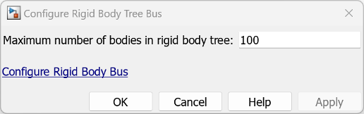
To configure the maximum number of bodies in a rigid body tree, click
Configure Rigid Body Tree Bus in the block mask to open the Configure
Rigid Body Tree Bus dialog box, and set the Maximum number of bodies in rigid
body tree parameter. The default value is 100.
To configure the maximum number of collisions for rigid bodies of the rigid body tree,
click Configure Rigid Body Bus in the Configure Rigid Body Tree Bus
dialog box to open the Configure Rigid Body Bus dialog box, and set the Maximum
number of collisions in rigid body parameter. The default value is
5.
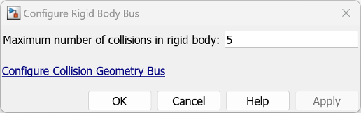
To configure the maximum number of vertices in the collision geometries of the rigid bodies, click Configure Collision Geometry Bus in the block mask to open the Configure Collision Geometry Bus dialog box. See Configure Collision Geometry Bus for more information.
Extended Capabilities
Version History
Introduced in R2026a