Generate Time-Optimal Trajectories with Constraints Using TOPP-RA Solver
This example shows how to generate trajectories that satisfy velocity and acceleration limits. The example uses the contopptraj function, which solves a constrained time-optimal path parametrized (TOPP) trajectory using reachability analysis (RA).
Background
This example solves a TOPP problem, which is a robotics problem in which the goal is to find the fastest way to traverse a path subject to system constraints. In this example, you use the contopptraj function which solves a TOPP problem subject to velocity and acceleration constraints by using a method based on reachability analysis (RA), coined TOPP-RA [1]. Other methods to solve TOPP problems rely on numerical integration (NI) or convex optimization (CO). Applications of TOPP include:
Re-timing a joint-space trajectory for a manipulator to meet manufacturer-provided kinematic constraints.
Generating a joint-space trajectory that returns fast and optimal trajectories given a planned path.
Optimizing the traversal of a mobile robot path in SE(3) given limits on its motion.
You can use the contopptraj function in these ways:
Generate a trajectory that connects waypoints while satisfying velocity and acceleration limits. In this case, use a minimum jerk trajectory as the initial guess. For more information, see Create Kinematically Constrained Trajectory.
Re-parameterize an existing trajectory while preserving its timing given velocity and acceleration constraints. The path, which consists of waypoints in the N-dimensional input space, is a trajectory of any kind. The
contopptrajfunction then scales how the robot navigates the path in the same time, mapping the existing trajectory to a new one that solves the TOPP problem.
In this example, you update an existing trajectory that connects five 2-D waypoints. The initial path is interpolated with an initial trajectory based on a quintic polynomial, which provides the shape. You then use the contopptraj function to apply velocity and acceleration limits to the initial path.
Define Waypoints and Initial Trajectory
Both trajectories connect the same set of waypoints, subject to a set of velocity and acceleration limits. Specify the waypoints.
waypts = (deg2rad(30))*[-1 1 2 -1 -1.5; 1 0 -1 -1.1 1];
Different trajectories have different geometric and kinematic attributes, which affects how they navigate a path in space. The Choose Trajectories for Manipulator Paths example illustrates some differences between the various trajectory functions provided in Robotics System Toolbox™.
For this example, use a quintic polynomial trajectory to connect the waypoints. The quintic polynomial connects segments by using smooth velocity and acceleration profiles.
tpts = [0 1 2 3 5];
timeVec = linspace(tpts(1),tpts(end),100);
[q1,qd1,qdd1,pp1] = quinticpolytraj(waypts,tpts,timeVec);
Refine Trajectory Using Constrained TOPP-RA Solver
The quintic polynomial produces an output that, with default parameters, stops at each waypoint. You can use a TOPP-RA solver to compute the fastest possible way to traverse the path while still stopping at each waypoint, given bounded velocity and acceleration. Use the contopptraj function to generate a trajectory that traverses the initial path as quickly as possible while satisfying the specified velocity and acceleration limits.
vellim = [-40 40; -25 25];
accellim = [-10 10; -10 10];
[q2,qd2,qdd2,t2] = contopptraj(pp1,vellim,accellim,numsamples=100);
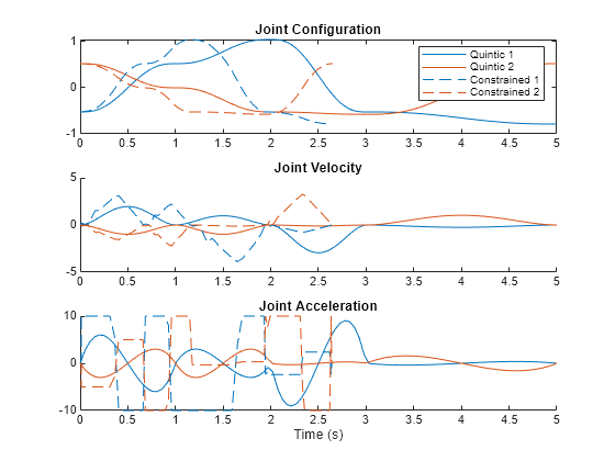
Plot the initial and modified trajectory on the same plot. Notice how the TOPP-RA solver speeds up the trajectory while still satisfying the known constraints.
% Create a figure and adjust the color order so that the second two lines
% have the same color as the associated first two lines
figure
c = colororder("default");
c(3:4,:) = c(1:2,:);
colororder(c)

% Plot results
subplot(3,1,1)
plot(timeVec,q1);
hold on
plot(t2,q2,"--")
legend("Quintic 1","Quintic 2","Constrained 1","Constrained 2")
title("Joint Configuration")
xlim([0 tpts(end)])

subplot(3,1,2)
hold on
plot(timeVec,qd1)
plot(t2,qd2,"--")
title("Joint Velocity")
xlim([0 tpts(end)])

subplot(3,1,3)
hold on
plot(timeVec,qdd1)
plot(t2,qdd2,"--")
title("Joint Acceleration")
xlabel("Time (s)")
xlim([0 tpts(end)])
References
Pham, Hung, and Quang-Cuong Pham. “A New Approach to Time-Optimal Path Parameterization Based on Reachability Analysis.” IEEE Transactions on Robotics, 34, no. 3 (June 2018): 645–59. https://doi.org/10.1109/TRO.2018.2819195.