Solve Inverse Kinematics for Closed Loop Linkages
Closed loop linkages are widely used in automobiles, construction and manufacturing machines, and in robot manipulation. Although you cannot directly model closed-loop linkages with the rigidBodyTreeImportInfo object in Robotics System Toolbox™, you can still study the kinematics of closed-loop systems by combining a rigid body tree with constraints that mimic loop-closing joints. The constraintRevoluteJoint, constraintPrismaticJoint, and constraintFixedJoint constraint objects enable you to model loop-closing revolute, prismatic, and fixed joints, respectively. To kinematically model closed-loop linkages, use the constraints with a generalizedInverseKinematics solver to constrain the solutions to act as desired.
This example shows how to model a four-bar linkage, a widely used closed-loop linkage, using the rigidBodyTree and constraintRevoluteJoint objects, and the generalizedInverseKinematics System object™.
Four-Bar Linkage as Rigid Body Tree with Revolute Joint Constraint
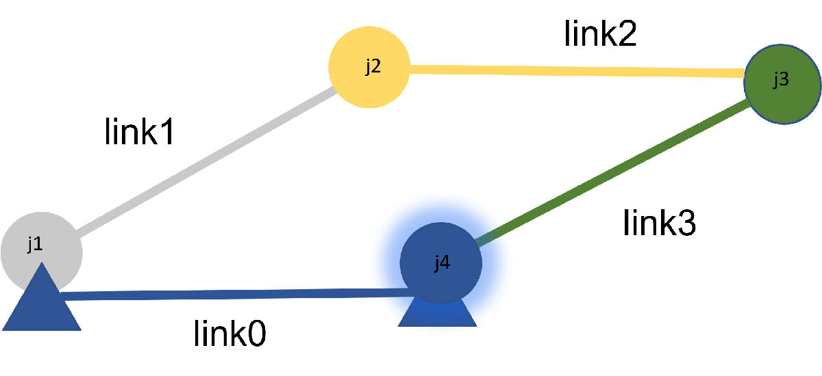
This figure shows a four-bar linkage. The highlighted joint is a loop-closing revolute joint.
You can create a rigid body tree corresponding to the four-bar linkage, which consists of joints , , and , and is constrained with a revolute joint constraint that acts as a fourth joint, . This figure shows the reference frames of the links of the rigid body tree in an unconstrained joint configuration. The frames of the links are located at their respective joints. The frame corresponding to the base body of the rigid body tree, , is represented by the black arrows.
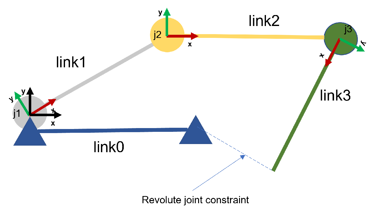
Create the four bar linkage by starting from a three-joint rigidBodyTree. Add a collision body to the base joint for 'link0'.
fourBarLinkageTree = exampleHelperFourBarLinkageTree();
Visualize the rigid body tree in an unconstrained configuration.
figure(Name="Rigid Body Tree Unconstrained As Four-Bar Linkage",Visible="on")
unconstrainedConfig = [pi/4 -pi/4 -110*pi/180];
show(fourBarLinkageTree, unconstrainedConfig, Collisions="on", Frames="on");
title("Rigid Body Tree Unconstrained as Four-Bar Linkage")
view([0 0 pi/2])
Intermediate Frames of Constraints
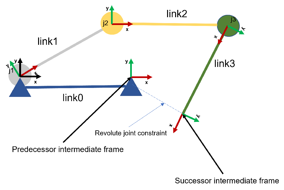
Revolute joint constraints constrain two intermediate frames. Each frame corresponds to the predecessor and the successor body. This figure below shows which intermediate frames to constrain to mimic the loop-closing joint.
Add these frames to the rigidBodyTree.
predjntframe = 'predecessorFrame';
succjntframe = 'successorFrame';
fourBarLinkageTree.Base.addFrame(predjntframe,'link0',trvec2tform([1 0 0]));
fourBarLinkageTree.Bodies{end}.addFrame(succjntframe,'link3',trvec2tform([1 0 0]));
Visualize the added frames
exampleHelperAddFrameVisual(fourBarLinkageTree.Base,predjntframe);
exampleHelperAddFrameVisual(fourBarLinkageTree.Bodies{end},succjntframe);

hold on;
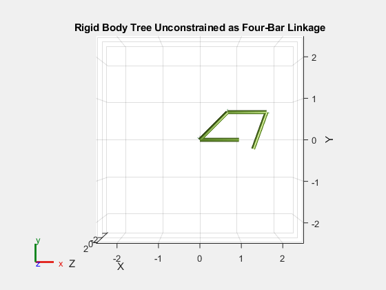
show(fourBarLinkageTree, unconstrainedConfig, Collisions="on", Frames="on");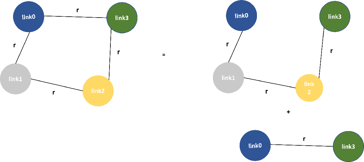
Connectivity Graph of Four-Bar Linkage
One way to approach the modeling of closed-loop linkages is by using connectivity graphs. This approach models the kinematic linkage using a graph whose vertices are the links of the linkage, and an edge between links represents the joint between them.
Using this representation, the goal of modeling the closed-loop linkage as a rigid body tree with joint constraints is to remove edges from the graph so that the graph becomes a tree. A tree is a graph with no loops, which instead uses constraints to enforce the removed edges.
In the connectivity graph, the difference between the four-bar linkage and its equivalent rigid body tree representation is that the rigid body tree needs a loop-closing joint constraint from to .
Set Up Inverse Kinematics Solver
The four-bar linkage is a one degree-of-freedom linkage, and is driven by the crank link, . Given a crank position specified by the value of joint , the generalized inverse kinematics solver outputs the joint positions corresponding to joints and .
Create an instance of the generalized inverse kinematics solver. For this task, the solver requires two constraint objects, constraintJointBounds and constraintRevoluteJoint.
solverFourBarLinkage = generalizedInverseKinematics(...
    RigidBodyTree=fourBarLinkageTree, ...
    ConstraintInputs={'jointbounds','revolutejoint'});

% Disable random restarts for repeatable IK solutions
solverFourBarLinkage.SolverParameters.AllowRandomRestart = false;
solverFourBarLinkage.SolverParameters.StepTolerance = 1e-14;
Define the revolute joint constraint between and at the 'successorFrame' and 'predecessorFrame' respectively.
% Revolute joint constraint between "link3" and "link0"
cRevolute = constraintRevoluteJoint("link3","link0",...
    "SuccessorTransform",succjntframe,...
    "PredecessorTransform",predjntframe);
To ensure that the crank position is fixed with respect to the solution, you must implement a joint bounds constraint. The elements of the Weights property of the joint bounds constraint corresponds to a joint position in the joint configuration of the rigid body tree. In this case, only joint has a non-zero weight, as it is the joint that we want to constrain.
% Joint bounds constraint to fix the crank position.
activeJointConstraint = constraintJointBounds(fourBarLinkageTree);
activeJointConstraint.Weights = [1 0 0];
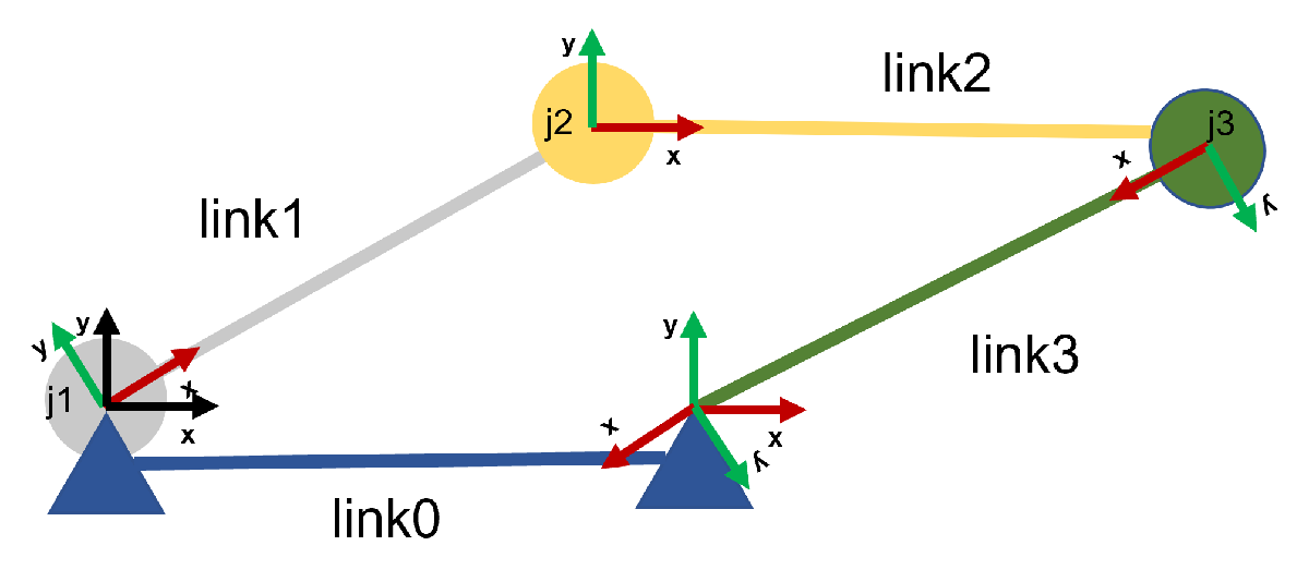
If you constrain the intermediate frames, they co-locate. This figure shows a constrained configuration that corresponds to the unconstrained configuration.

Visualize Constrained Motion
The joint position, theta, of the crank drives the linkage. For a discrete set of crank positions in the interval, the solver solves for joint positions in the rigid body tree such that it behaves like a four-bar linkage. This code visualizes the constrained rigid body tree for every crank position, theta.
For the initial crank position, , guess an initial constrained configuration for the solver. The visualization loop overwrites this value.
constrainedConfig = [pi/2 0 pi/3];
Initialize the figure for visualization.
figure(Name="Rigid Body Tree Constrained As Four-Bar Linkage",Visible="on")
ax = show(fourBarLinkageTree,constrainedConfig, ...
    PreservePlot=false, ...
    FastUpdate=true, ...
    Collisions="on");
title("Rigid Body Tree Constrained as Four-Bar Linkage")
Visualize the four-bar linkage for a specified crank position.
for theta = linspace(pi/2,5*pi/2,101)
    % Fix the crank position to "theta" in the solver-generated constrained
    % config. This is done by setting identical upper and lower values for
    % the joint bounds constraint.
    config = [theta constrainedConfig(2) constrainedConfig(3)];
    activeJointConstraint.Bounds(1,:) = [theta theta];
    constrainedConfig = solverFourBarLinkage(config,activeJointConstraint,cRevolute);

    % Visualize the constrained rigid body tree and the
    % predecessor and successor intermediate frames of the constraint.
    show(fourBarLinkageTree,constrainedConfig, ...
        PreservePlot=false, ...
        FastUpdate=true, ...
        Collisions="on");
    view([0 0 pi/2]);
    drawnow;
end
See Also
generalizedInverseKinematics | Inverse Kinematics Designer