constraintFixedJoint
Description
The constraintFixedJoint object describes a closed-loop fixed
joint constraint between a successor and predecessor body on the same rigidBodyTree. The constraint is satisfied when there is no relative orientation,
and the origins of the frames coincide. This constraint allows no relative motion between the
intermediate frames when satisfied.
Creation
Syntax
Description
fixedConst = constraintFixedJoint(successorbody,predecessorbody)fixedConst, that represents a
constraint between the specified successor body successorbody and
predecessor body predecessorbody of the joint. The
successorbody and predecessor arguments set
the SuccessorBody and PredecessorBody
properties, respectively.
fixedConst = constraintFixedJoint(___,Name=Value)
Properties
Examples
Create a revolute, prismatic, and fixed joint constraints for a simple rigid body tree.
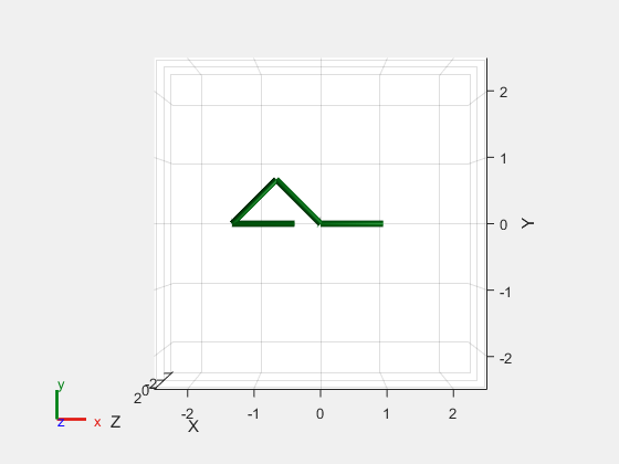
Use the exampleHelperFourBarLinkageTree helper function to create a simple robot model to demonstrate the closed-loop constraints.
rbt = exampleHelperFourBarLinkageTree;
show(rbt,Collisions="on");
view([0 0 pi])
xlim([-1 4])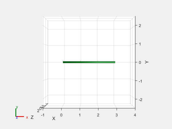
Revolute Joint Constraint
To demonstrate a revolute joint constraint, create a four-bar linkage by connecting the end of the last link, link3, and the first link, link0.
Create a generalized inverse kinematics solver with a revolute joint constraint and a joint bounds constraint.
gikSolverWithRevoluteJointConstraint = generalizedInverseKinematics(RigidBodyTree=rbt, ...
    ConstraintInputs={'revolute','jointbounds'});
To ensure repeatable IK solutions, disable random restarts.
gikSolverWithRevoluteJointConstraint.SolverParameters.AllowRandomRestart = false;
theta = pi/2+pi/4;
Fix the first joint by setting theta as both the minimum and maximum bound.
activeJointConstraint = constraintJointBounds(rbt);
activeJointConstraint.Weights = [1 0 0];
activeJointConstraint.Bounds(1,:) = [theta theta];
Create a revolute joint constraint with successor and predecessor bodies set to the last link link3 and the first link link0, respectively. Specify predecessor and successor transforms that create intermediate frames 1 meter away, in the X-axis, from their respective body. Once defined, these intermediate frames move such that their frame origins coincide when their Z-axes align.
cRev = constraintRevoluteJoint("link3","link0", ...
    PredecessorTransform=trvec2tform([1 0 0]), ...
    SuccessorTransform=trvec2tform([1 0 0]));
Provide [theta 0 0] as an initial guess to the solver, along with the constraints.
qConst = gikSolverWithRevoluteJointConstraint([theta 0 0],cRev,activeJointConstraint);
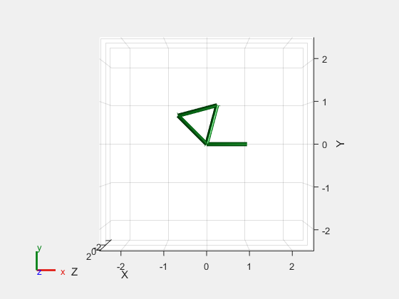
Visualize the robot to see the robot acting as a four-bar linkage. If the first joint rotates, the solver tries to keep the intermediate frames of the revolute joint constraint coincident, acting as a joint and resulting in four-bar motion.
figure(Name="Revolute Joint Constraint")
show(rbt,qConst,Collisions="on")
view([0 0 pi])
Prismatic Joint Constraint
Use a prismatic joint constraint to create a slider-crank. Create a new solver with a prismatic joint constraint and a joint bounds constraint.
gikSolverWithPrismaticJointConstraint = generalizedInverseKinematics(RigidBodyTree=rbt, ...
    ConstraintInputs={'prismatic','jointbounds'});
gikSolverWithPrismaticJointConstraint.SolverParameters.AllowRandomRestart=false;
Create the prismatic joint constraint with link3 and link0 as the successor and predecessor bodies, respectively, and set the predecessor transform such that the predecessor intermediate frame is 1 meter away on the X-axis and rotated pi/2 in the Y-axis from the predecessor body frame.
cPris=constraintPrismaticJoint("link3","link0",PredecessorTransform=trvec2tform([1 0 0])*eul2tform([0 pi/2 0]));
Provide [theta 0 0] as an initial guess to the solver along with the constraints.
qConst = gikSolverWithPrismaticJointConstraint([theta 0 0],cPris,activeJointConstraint);
Visualize the robot to see the robot acting as a slider-crank. If the first joint rotates, the solver tries to keep the intermediate frames of the prismatic joint constraint coincident, acting as a joint and resulting in slider-crank motion.
figure(Name="Prismatic Joint Constraint")
show(rbt,qConst,Collisions="on")
view([0 0 pi])
Fixed Joint Constraint
To demonstrate a fixed joint constraint, create a triangle with the links that is preserved when the first joint moves. Create a new solver with a fixed joint constraint.
gikSolverWithFixedJointConstraint = generalizedInverseKinematics(RigidBodyTree=rbt, ...
    ConstraintInputs={'fixed'});
Create the fixed joint constraint with link3 and link0 as the successor and predecessor bodies, respectively, and set the successor transform such that the predecessor intermediate frame is 1 meter away on the X-axis from the predecessor body frame.
cFix = constraintFixedJoint("link3","link1",SuccessorTransform=trvec2tform([1 0 0]));
Set the weight of the orientation constraint of the fixed joint constraint to 0.
cFix.Weights = [1 0];
[qConst,solInfo] = gikSolverWithFixedJointConstraint([theta 0.1 0],cFix);
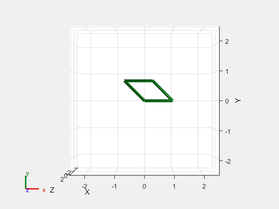
Visualize the robot to see how the fixed constraint joint acts on the robot frame. If the first joint rotates, the solver tries to keep the intermediate frames of the fixed joint constraint coincident, acting as a fixed joint.
figure(Name="Fixed Joint Constraint")
show(rbt,qConst,Collisions="on")
view([0 0 pi])