Mixed-Sensitivity Loop Shaping

Mixed-sensitivity loop shaping lets you design an H_∞ controller by simultaneously shaping the frequency responses for tracking and disturbance rejection, noise reduction and robustness, and controller effort. This technique is a useful way to balance the necessary tradeoff between performance and robustness (see Loop Shaping for Performance and Robustness). To use this technique, you convert your desired responses into up to three weighting functions that the mixsyn command uses to synthesize the controller.

Problem Setup

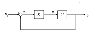
mixsyn designs a controller K for your plant G, assuming the standard control configuration of the following diagram.

Plant G in negative unit feedback control configuration with controller K

To do so, the function appends the weighting functions you provide, W₁(s), W₂(s), and W₃(s), to the control system, as shown in the following diagram.

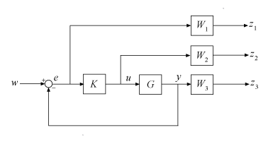
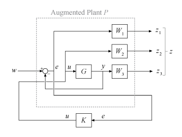
Weighting functions for mixsyn. Output z1 is the error signal weighted by W1. Output z2 is the control signal u weighted by W2. Output z3 is the plant output y weighted by W3.

mixsyn treats the problem as an H_∞ synthesis problem (see hinfsyn). It analyzes the weighted control system as LFT(P,K), where P is an augmented plant P such that {z;e} = P{w;u}, as shown in the following diagram.

Closed-loop control system with the augmented plant P that includes the weighting functions. P has inputs {w,u} and outputs {z,e} where z = {z1,z2,z3}. P is interconnected with controller K in an LFT configuration, where K has input e and output u.

The transfer function from w to z can be expressed as

$M (s) = [\begin{matrix} W_{1} S \\ W_{2} K S \\ W_{3} T \end{matrix}],$

where

S = (I + GK)^–1 is the sensitivity function.
KS is the transfer function from w to u (the control effort).
T = (I – S) = GK(I + GK)^–1 is the complementary sensitivity function.

mixsyn seeks a controller K that minimizes ||M(s)||_∞, the H_∞ norm (peak gain) of M. To do so, it invokes hinfsyn on the augmented plant P = augw(G,W1,W2,W3).

Choose Weighting Functions

For loop gain L = GK, to achieve good reference tracking and disturbance rejection, you typically want high loop gain at low frequency. To achieve robustness and attenuation of measurement noise, you typically want L to roll off at high frequency. This loop shape is equivalent to small S at low frequency and small T at high frequency.

For mixed-sensitivity loop shaping, you choose weighting functions to specify those target shapes for S and T as well as the control effort KS. The H_∞ design constraint,

${‖ M (s) ‖}_{\infty} = {‖ [\begin{matrix} W_{1} S \\ W_{2} K S \\ W_{3} T \end{matrix}] ‖}_{\infty} \leq 1,$

means that

$\begin{matrix} {‖ S ‖}_{\infty} \leq | W_{1}^{- 1} | \\ {‖ K S ‖}_{\infty} \leq | W_{2}^{- 1} | \\ {‖ T ‖}_{\infty} \leq | W_{3}^{- 1} | . \end{matrix}$

Therefore, you set the weights equal to the reciprocals of the desired shapes for S, KS, and T. In particular,

For good reference-tracking and disturbance-rejection performance, choose W₁ large inside the control bandwidth to obtain small S.
For robustness and noise attenuation, choose W₃ large outside the control bandwidth to obtain small T.
To limit control effort in a particular frequency band, increase the magnitude of W₂ in this frequency band to obtain small KS.

mixsyn returns the minimum ||M(s)||_∞ in the output argument gamma. For the returned controller K, then,

$\begin{matrix} {‖ S ‖}_{\infty} \leq γ | W_{1}^{- 1} | \\ {‖ K S ‖}_{\infty} \leq γ | W_{2}^{- 1} | \\ {‖ T ‖}_{\infty} \leq γ | W_{3}^{- 1} | . \end{matrix}$

If you do not want to restrict control effort, you can omit W₂. In that case, mixsyn minimizes the H_∞ norm of

$M (s) = [\begin{matrix} W_{1} S \\ W_{3} T \end{matrix}] .$

You can use makeweight to create weighting functions with the desired gain profiles. The following example illustrates how to choose and create weighting functions for controller design with mixsyn.

Numeric Considerations

Do not choose weighting functions with poles very close to s = 0 (z = 1 for discrete-time systems). For instance, although it might seem sensible to choose W₁ = 1/s to enforce zero steady-state error, doing so introduces an unstable pole that cannot be stabilized, causing synthesis to fail. Instead, choose W₁ = 1/(s + δ). The value δ must be small but not very small compared to system dynamics. For instance, for best numeric results, if your target crossover frequency is around 1 rad/s, choose δ = 0.0001 or 0.001. Similarly, in discrete time, choose sample times such that system and weighting dynamics are not more than a decade or two below the Nyquist frequency.

Mixed-Sensitivity Loop-Shaping Controller Design

Open Live Script

Load a plant model for a mixed-sensitivity $H_{\infty}$ controller design. This two-input, two-output, six-state model is described in the example Loop-Shaping Controller Design.

load mixsynExampleData G
size(G)

State-space model with 2 outputs, 2 inputs, and 6 states.

To design a controller for performance and robustness, shape the sensitivity and complementary sensitivity functions. Choose weights that are the inverse of the desired shapes.

To achieve good reference-tracking and disturbance-rejection performance, shape S to be small inside the control bandwidth, which means choosing W1 large at low frequency, rolling off at high frequency. For this example, specify W1 with:

Low-frequency gain of about 30 dB (33 in absolute units)
High-frequency gain of about –6 dB (0.5 in absolute units)
0 dB crossover at about 5 rad/s.

W1 = makeweight(33,5,0.5);

For robustness and noise attenuation, shape T to be small outside the control bandwidth, which means choosing W3 large at high frequency.

W3 = makeweight(0.5,20,20);

Examine both weighting functions. Their inverses are the target shapes for S and T.

bodemag(W1,W3)
yline(0,'--');
legend('W1','W3','0 dB');
grid on

MATLAB figure

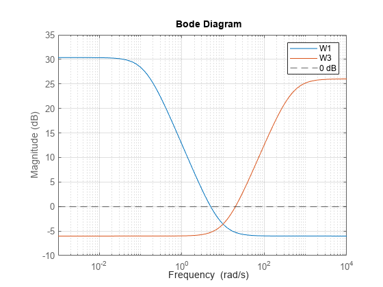
Because S + T = I, mixsyn cannot make both S and T small (less than 0 dB) in the same frequency range. Therefore, when you specify weights, there must be a frequency band in which both W1 and W3 are below 0 dB.

Use mixsyn to compute the optimal mixed-sensitivity controller with these weights. For this example, impose no penalty on controller effort by setting W2 to [].

[K,CL,gamma] = mixsyn(G,W1,[],W3);
gamma

gamma = 
0.7331

The resulting gamma, which is the peak singular value across all frequencies, is well below 1, indicating that the closed-loop system meets the design requirements. Examine the resulting system responses. First, compare the resulting sensitivity S and complementary sensitivity T to the corresponding weighting functions W1 and W3.

L = G*K;
I = eye(size(L));
S = feedback(I,L); 
T= I-S;

sigma(S,'b',W1,'b--',T,'r',W3,'r--',{0.1,1000})
legend('S','W1','T','W3');

MATLAB figure

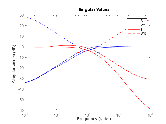
The plot shows that S and T achieve the desired loop shape, where S is large inside the control bandwidth and a is small outside the control bandwidth.

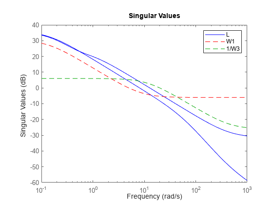
To see how mixed-sensitivity loop-shaping achieves the goals of classic loop shaping, compare the open-loop response L to the weighting functions. L ~ W1 where W1 is large, and L ~ 1/W3 where W3 is large.

sigma(L,'b',W1,'r--',1/W3,'g--',{0.1,1000})
legend('L','W1','1/W3');

MATLAB figure

Mixed-Sensitivity Loop Shaping

Problem Setup

Choose Weighting Functions

Numeric Considerations

Mixed-Sensitivity Loop-Shaping Controller Design

See Also

Related Topics