Loop Shaping for Performance and Robustness

Performance and robustness requirements can often be expressed in terms of the open-loop response gain. For example, high gain at low frequencies reduces steady-state offsets and improves disturbance rejection. Similarly, high-frequency rolloff improves stability where the plant model is uncertain or inaccurate. Loop shaping is an approach to control design in which you determine a suitable profile for the open-loop system response and design a controller to achieve that shape.

Tradeoff Between Performance and Robustness

The uncertainty in your plant model can be a limiting factor in determining what you can achieve with feedback. High loop gains can attenuate the effects of plant model uncertainty and reduce the overall sensitivity of the system to disturbances. But if your plant model uncertainty is so large that you do not even know the sign of your plant gain, then you cannot use large feedback gains without the risk of the system becoming unstable.

For this reason, most controller designs involve a tradeoff between performance and robustness against uncertainty. Robust Control Toolbox™ commands for loop-shaping controller design let you determine the tradeoff that best meets the requirements of your system.

loopsyn — Designs a stabilizing controller that shapes the open-loop response to approximate the target loop shape that you provide. You can adjust the balance between performance and robustness.
mixsyn — Controller design optimized for performance. This function allows you more precise specification of the shapes of different loop responses.
ncfsyn — Controller design optimized for robustness (stability margin). You provide weighting functions that shape the plant to a desirable profile.

The performance optimization of mixsyn tends to produce plant-inverting designs, which can be less robust. In particular, mixsyn designs can be fragile for ill-conditioned MIMO plants and for plants with structured uncertainty, such as uncertainty on the damping and natural frequency of resonant modes. In contrast, ncfsyn deters control strategies like plant inversion that rely on exact knowledge of the plant poles and zeroes. Thus ncfsyn adds some of the robustness to structured uncertainty that is missing in mixsyn designs. By combining elements of both ncfsyn and mixsyn, the loopsyn approach can provide robustness to both structured and unstructured uncertainty while also providing good performance.

Choosing a Target Loop Shape

Here are some basic design tradeoffs to consider when choosing a target loop shape.

Robust Stability. Use a target loop shape with gain as low as possible at high frequencies where typically your plant model is so poor that its phase angle is completely inaccurate, with errors approaching ±180° or more.
Performance. Use a target loop shape with gain as high as possible at frequencies where your model is good. Doing so ensures good reference tracking and good disturbance attenuation.
Crossover and Rolloff. Use a target loop shape with its 0 dB crossover frequency ω_c between the previous two frequency ranges. Ensure that the target loop shape rolls off with a slope between –20 dB/decade and –30 dB/decade near ω_c. This rolloff helps keep phase lag approximately between –130° and –90° near crossover for good phase margins.

Keep these principles in mind when choosing your target loop shape for loopsyn or the shaping filters for ncfsyn. For further details about choosing weighting functions for mixsyn, see Mixed-Sensitivity Loop Shaping.

Limitations on Control Bandwidth

Other considerations that might affect your choice of loop shape are the unstable poles and zeros of the plant, which impose fundamental limits on your 0 dB crossover frequency ω_c (see [1]). For instance, ω_c must be greater than the natural frequency of any unstable pole of the plant, and smaller than the natural frequency of any unstable zero of the plant.

$\max_{Re (p_{i}) > 0} | p_{i} | < ω_{c} < \min_{Re (z_{i}) > 0} | z_{i} | .$

If you do not take care to choose a target loop shape that conforms to these fundamental constraints, then you might not achieve good results. For instance, loopsyn computes the optimal loop-shaping controller K for a target loop shape Gd that does not meet this requirement, but the resulting response L = G*K might have a poor fit to the target loop shape Gd, and consequently it might be impossible to meet your performance goals.

Additionally, because plant uncertainty typically increases with frequency, the bandwidth that you can reliably achieve is limited. For instance, consider an approximate model G₀ of a SISO plant G. You can express the uncertainty in this plant as a multiplicative uncertainty Δ _M, such that $G = G_{0} (1 + Δ_{M})$ . The uncertainty is bounded at each frequency such that |Δ _M(jω)| ≤ β(ω), where β(ω) is the percentage of model uncertainty. Typically, β(ω) is small at low frequencies (accurate model) and increases at high frequencies (inaccurate model). The frequency where β(ω) = 2 marks a critical threshold beyond which you have insufficient information about the plant to reliably design a feedback controller. With such a 200% model uncertainty, the model provides no indication of the phase angle of the true plant, which means that the only way you can reliably stabilize your plant is to ensure that the loop gain is less than 1. Allowing for an additional factor of two margin for error, your control system bandwidth is essentially limited to the frequency range over which your multiplicative plant uncertainty Δ _M has gain magnitude |Δ _M|<1.

Loop Shapes, Performance, and Robustness

For a deeper understanding of the relationship between loop shapes, performance, and robustness, consider the multivariable feedback control system shown in the following figure.

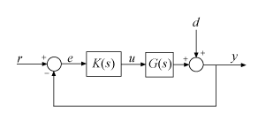
Unit negative feedback control architecture with reference signal r, error signal e, controller K(s), control signal u, plant G(s), plant disturbance d, and output y.

To quantify the multivariable stability margins and performance of such systems, you can use the closed-loop sensitivity function S and complementary sensitivity function T, defined as

$\begin{array}{l} S (s) \overset{d e f}{=} {(I + L (s))}^{- 1} \\ T (s) \overset{d e f}{=} L (s) {(I + L (s))}^{- 1} = I - S (s), \end{array}$

where L(s) is the open-loop transfer function

$L (s) = G (s) K (s) .$

Specifying a target shape G_d(s) for the open-loop transfer function L(s) is equivalent to imposing constraints on the singular values of the sensitivity S(s) and complementary sensitivity T(s). For instance, for a target loop shape with high gain at low frequency, the condition $\underline{σ} (L (s)) > \underline{σ} (G_{d} (s)) ≫ 1$ is equivalent to $\bar{σ} (S (s)) < 1 / \underline{σ} (G_{d} (s))$ , where $\bar{σ}$ and $\underline{σ}$ denote the largest and smallest singular values, respectively. Similarly, for a target loop shape with low gain at high frequency, $\bar{σ} (L (s)) < \bar{σ} (G_{d} (s)) ≪ 1$ is equivalent to $\bar{σ} (T (s)) < \bar{σ} (G_{d} (s))$ .

When using loopsyn, you specify G_d(s) directly, and loopsyn approximately imposes these constraints on the sensitivity and complementary sensitivity. For mixsyn, you specify weighting functions W₁(s) and W₃(s) such that W₁(s) matches 1/G_d(s) at low frequency and is smaller than 1 elsewhere, and W₃(s) matches G_d(s) at high frequency and is smaller than 1 elsewhere. (See Mixed-Sensitivity Loop Shaping). Then mixsyn approximately imposes the constraints $\bar{σ} (S) < | W_{1}^{- 1} |$ and $\bar{σ} (T) < | W_{3}^{- 1} |$ , which roughly enforce the loop shape G_d.

Additionally, robustness to multiplicative plant uncertainty is equivalent to imposing a small-gain constraint on T(s) (see [1], page 342). Thus, enforcing rolloff in the loop shape G_d (or equivalently, $\bar{σ} (T) < | W_{3}^{- 1} |$ ) provides some robustness against unmodeled plant dynamics at high frequency.

Guaranteed Gain and Phase Margins

If you are more comfortable with classical single-loop concepts, you can use the important connections between the multiplicative stability margins predicted by the gain of T(s) and those predicted by classical M-circles, as found on the Nichols chart. In the SISO case, the largest singular value of T(s) is just the peak gain, given by:

$| T (s) | = | \frac{L (s)}{1 + L (s)} | .$

This quantity is the same quantity you obtain from Nichols chart M-circles. The H_∞ norm ${‖ T ‖}_{\infty}$ (see hinfnorm) is a multiloop generalization of the closed-loop resonant peak magnitude which, as classical control experts will recognize, is closely related to the damping ratio of the dominant closed-loop poles. You can relate ${‖ T ‖}_{\infty}$ and ${‖ S ‖}_{\infty}$ to the classical gain margin G_M and phase margin θ_M in each feedback loop of the multivariable feedback system illustrated in the previous section, via the formulas:

$\begin{array}{l} G_{M} \geq 1 + \frac{1}{{‖ T ‖}_{\infty}} \\ G_{M} \geq 1 + \frac{1}{1 - \frac{1}{{‖ S ‖}_{\infty}}} \\ θ_{M} \geq 2 \sin^{- 1} (\frac{1}{2 {‖ T ‖}_{\infty}}) \\ θ_{M} \geq 2 \sin^{- 1} (\frac{1}{2 {‖ S ‖}_{\infty}}) . \end{array}$

(See [2].) These formulas are valid provided ${‖ S ‖}_{\infty}$ and ${‖ T ‖}_{\infty}$ are larger than 1, as is normally the case. The margins apply even when the gain perturbations or phase perturbations occur simultaneously in several feedback channels.

The infinity norms of S and T also yield gain-reduction tolerances. The gain-reduction tolerance g_M is defined to be the minimal amount by which the gains in each loop would have to be decreased in order to destabilize the system. Upper bounds on g_M are as follows:

$\begin{array}{l} g_{M} \leq 1 - \frac{1}{{‖ T ‖}_{\infty}} \\ g_{M} \leq \frac{1}{1 + \frac{1}{{‖ S ‖}_{\infty}}} . \end{array}$

For more information about the relation between sensitivity functions and gain and phase margins, see [3].

References

[1] Skogestad, Sigurd, Ian Postlethwaite. Multivariable Feedback Control: Analysis and Design. Chichester; New York: Wiley, 1996.

[2] Lehtomaki, N., N. Sandell, and M. Athans. "Robustness Results in Linear-Quadratic Gaussian Based Multivariable Control Designs." IEEE Transactions on Automatic Control 26, no.1 (February 1981): 75–93.

[3] Seiler, Peter, Andrew Packard, and Pascal Gahinet. “An Introduction to Disk Margins [Lecture Notes].” IEEE Control Systems Magazine 40, no. 5 (October 2020): 78–95.