loopsyn

Consider the following plant.

s = zpk('s');
G = (s-10)/(s+100);

Design a controller that yields a closed-loop step response with a rise time of about 4 s. A simple target loop shape for this requirement is Gd = wc/s, where the target crossover frequency wc is related to the desired rise time by t = 2/wc.

wc = 0.5; 
Gd = wc/s;

Obtain the controller using loopsyn.

[K,CL,gamma] = loopsyn(G,Gd);
gamma

gamma = 
1.1744

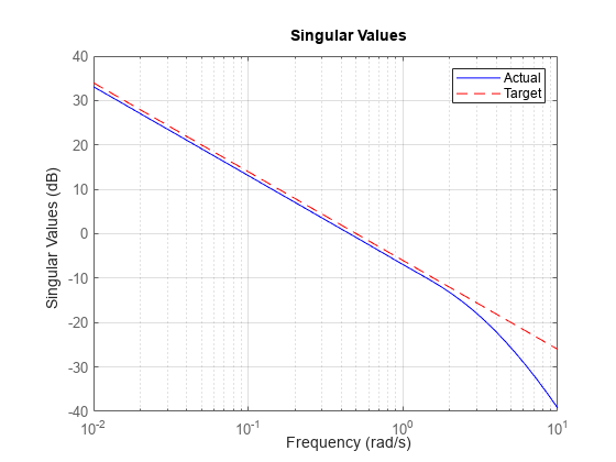
This value of gamma is close to 1, indicating a fairly good match between the achieved loop shape and the target loop shape. Compare the achieved open-loop response G*K with the desired response Gd.

sigma(G*K,"b",Gd,"r--",{0.01,10})
grid on
legend("Actual","Target")

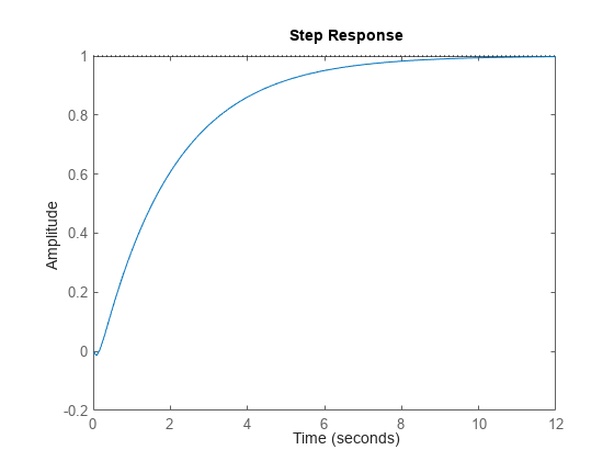
Examine the step response of the closed-loop system.

step(CL)

You can use the input argument alpha to specify how much loopsyn favors either performance (mixsyn design) or robustness (ncfsyn design). By default, loopsyn computes a balanced design, alpha = 0.5. To change the balance, change alpha. Consider the following plant and target loop shape.

G = tf(25,[1 10 10 10]); 
Gd = tf(0.5,[1 0]);

Design a loop-shaping controller that maximizes performance (minimizes gamma) subject to the constraint that the robustness (as determined by ncfmargin) is no worse than 75% of the maximum achievable robustness. To do so, set alpha to 0.75.

alpha = 0.75;
[K,CL,gamma,info] = loopsyn(G,Gd,alpha);

The maximum achievable robustness margin is returned in the info structure. Compare that value to the margin achieved by this controller. For ncfmargin, use the shaped plant and corresponding controller, also returned in info.

info.emax

ans = 
0.6474

ncfmargin(info.Gs,info.Ks)

ans = 
0.4880

These values confirm that the achieved robustness is 75% of the maximum robustness achievable by setting alpha = 1 for the pure ncfsyn design. For this plant, the alpha = 0.75 design yields a good match to the loop shape without sacrificing much robustness. Examine the performance and loop shape with this controller.

gamma

gamma = 
1.2149

sigma(G*K,"b",Gd,"r--",{0.01,10})
grid on
legend("Actual","Target")

For details on how to choose a good value of alpha for your application, see Loop-Shaping Controller Design.

When designing a controller for a MIMO system, if you specify a scalar Gd, then loopsyn applies the same target loop shape to all feedback channels. You can specify a different shape for each loop using a diagonal Gd of size Ny-by-Ny, where Ny is the number of feedback loops, or the number of outputs of G. Consider the following control system with a two-output, two-input plant.

s = tf('s');
G = [(1+0.1*s)/(1+s) 0.1/(s+2) ; 0 (s+2)/(s^2+s+3)];

Design a controller for this plant such as the first feedback channel has a crossover frequency of 1 rad/s and the second has a crossover frequency of 5 rad/s. To do so, create the loop shapes wc/s for each loop and use the append command to create the diagonal Gd.

wc = [1 5]; 
Gd = append(wc(1)/s,wc(2)/s);

Design the controller.

[K,CL] = loopsyn(G,Gd);

Compare the achieved loop shapes with the target loop shape.

bodemag(G*K,Gd,{0.1,100})
grid on
legend("Actual","Target")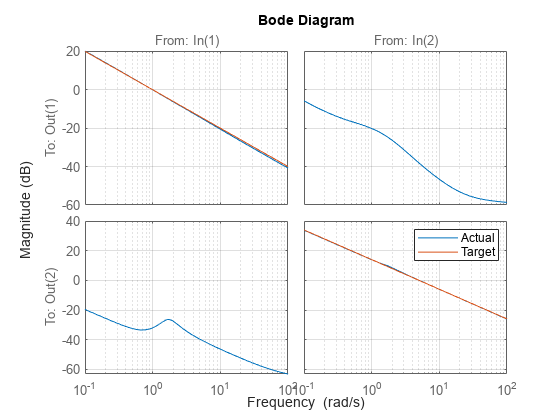

You can limit the order of the controller that loopsyn designs using the order argument. To specify a controller order, you must use a value of the parameter alpha such that 0 < alpha < 1.

Load a two-input, two-output plant.

load plant_loopsynOrderExample.mat G
size(G)

State-space model with 2 outputs, 2 inputs, and 7 states.

Design a controller for this plant with loop shape Gd = 0.5/s. Use alpha = 0.5 and let loopsyn select the controller order.

alpha = 0.5;
Gd = tf(0.5,[1 0]);
[K0,CL0,gamma0] = loopsyn(G,Gd,alpha); 
order(K0)

ans = 
5

loopsyn returns a controller with five states. Use loopsyn again to design a three-state controller.

ord = 3;
[K,CL,gamma,info] = loopsyn(G,Gd,alpha,ord); 
order(K)

ans = 
3

For this plant, reducing the controller order from five to three yields a small decrease in performance.

gamma0

gamma0 = 
1.0335

gamma

gamma = 
1.1828

Use a model-reduction command such as balred to identify suitable target orders to try for ord.

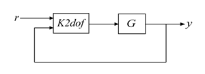
loopsyn can also provide a two-input, one output controller suitable for implementing the two-degree-of-freedom (2-DOF) architecture of the following illustration.

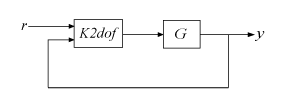
This architecture can be useful for mitigating the derivative kick that can occur when the reference signal changes. To obtain a controller suitable for this implementation, specify a plant and target loop shape, and call loopsyn.

G = tf(8625,[1 2.389 -5606]);
Gd = tf(80,[1 0])*tf(240,[1 240]);

[K,CL,gamma,info] = loopsyn(G,Gd);

The K2dof field of the info output contains the 2-DOF controller. For a plant with Nu inputs and Ny outputs, K2dof has Nu outputs and 2*Ny inputs. In this example, because G is SISO, K2dof has one output and two inputs.

K2dof = info.K2dof;
size(K2dof)

State-space model with 1 outputs, 2 inputs, and 4 states.

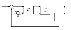
To use the controller, create a closed-loop system with the architecture shown previously.

L2dof = G*K2dof;
L2dof.InputName = {'r','y'};
L2dof.OutputName = 'y';
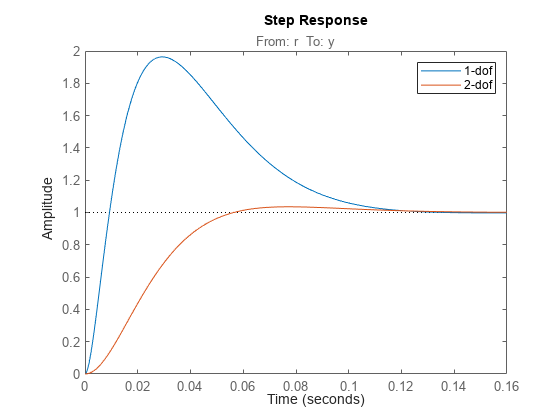
CL2dof = connect(L2dof,'r','y');

Compare the closed-loop step response with the two architectures. For this system, the 2-dof architecture substantially reduces the overshoot in the response.

step(CL,CL2dof)
legend("1-dof","2-dof")