Main Content

h2hinfsyn

Mixed H2/H synthesis with regional pole placement constraints

Description

[K,CL,normz,info] = h2hinfsyn(P,Nmeas,Ncon,Nz2,Wz,Name,Value) employs LMI techniques to compute an output-feedback control law u = K(s)y for the control problem of the following illustration.
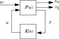
The LTI plant P has partitioned state-space form given by

x˙=Ax+B1w+B2u,z=C1x+D11w+D12u,z2=C2x+D21w+D22u,y=Cyx+Dy1w+Dy2u.

The resulting controller K:

  • Keeps the H norm G of the transfer function from w to z below the value you specify using the Name,Value argument 'HINFMAX'.

  • Keeps the H2 norm H of the transfer function from w to z2 below the value you specify using the Name,Value argument 'H2MAX'.

  • Minimizes a tradeoff criterion of the form

    W1G2+W2H2,

    where W1 and W2 are the first and second entries in the vector Wz.

  • Places the closed-loop poles in the LMI region that you specify using the Name,Value argument 'REGION'.

Use the input arguments Nmeas, Ncon, and Nz2 to specify the number of signals in y, u, and z2, respectively. You can use additional Name,Value pairs to specify additional options for the computation.

example

Examples

collapse all

Given a plant, design a controller such that the poles of the closed-loop system lie in the half-plane defined by Re(s) < –1.

You can define this region for pole-placement using the interactive lmireg command. To do so,

  1. Enter region = lmireg at the MATLAB® command line.

  2. Enter h to specify a half-plane constraint.

  3. Enter l to specify the left half-plane.

  4. Enter -1 to specify that the cutoff for the region is x0 = –1.

  5. Enter q to exit and create the LMI region.

The region created by this process is equivalent to the following commands. (For more information, see the lmireg reference page.)

RealPart = -1; 
region = [-2*RealPart + 1i 1]; 

Specify the plant model. For this example, use a two-input, three-output plant. Assume the plant contains one control signal and one measurement signal (nmeas = ncont = 1), and is partitioned such that these signals are the last input and output, respectively.

A = [1 0;2 1]; 
B = [1 1;1 0]; 
C = [1 1;1 1;1 1]; 
D = zeros(3,2);
P = ss(A,B,C,D);

Compute a controller for P using the LMI region to restrict the closed-loop pole locations. Apply an H2 norm constraint to one signal (Nz2 = 1) and give the H2 and H norms equal weight.

ncont = 1;
nmeas = 1;
Nz2 = 1 ;
Wz = [0 0];
[K,CL] = h2hinfsyn(P,nmeas,ncont,Nz2,Wz,'Region',region); 
 Solver for LMI feasibility problems L(x) < R(x)
    This solver minimizes  t  subject to  L(x) < R(x) + t*I
    The best value of t should be negative for feasibility

 Iteration   :    Best value of t so far 
 
     1                        7.368392
     2                      -95.362851

 Result:  best value of t:   -95.362851
          f-radius saturation:  0.009% of R =  1.00e+08
 

Confirm that the poles of the closed-loop system have Re(s) < –1.

pole(CL)
ans = 4×1 complex

  -1.6786 + 3.2056i
  -1.6786 - 3.2056i
  -1.5563 + 1.6678i
  -1.5563 - 1.6678i

You can push the closed-loop eigenvalues further left by changing RealPart. Or you can define other pole-placement regions. For instance, place the poles such that Re(s) falls in a strip of the complex plane –5 < Re(s) < –3. To define this region, use lmireg interactively to create reg1 specifying Re(s) > –5, and reg2 specifying Re(s) < –3. Then, enter region = lmireg(reg1,reg2) to define the intersection of these two regions. The following code is equivalent.

LeftRealPart = -5; 
RightRealPart = -3;
region = [-2*RightRealPart + 1i 0 1 0;
           0 2*LeftRealPart + 1i 0 -1];

Compute the new controller and confirm the locations of the closed-loop poles.

[K,CL] = h2hinfsyn(P,nmeas,ncont,Nz2,Wz,'Region',region); 
 Solver for LMI feasibility problems L(x) < R(x)
    This solver minimizes  t  subject to  L(x) < R(x) + t*I
    The best value of t should be negative for feasibility

 Iteration   :    Best value of t so far 
 
     1                       17.688394
     2                        1.074621
     3                      -13.502955

 Result:  best value of t:   -13.502955
          f-radius saturation:  0.048% of R =  1.00e+08
 
pole(CL)
ans = 4×1 complex

  -3.7864 + 4.9210i
  -3.7864 - 4.9210i
  -3.7752 + 3.6186i
  -3.7752 - 3.6186i

Input Arguments

collapse all

Plant, specified as an LTI model such as a tf or ss model. P must be a continuous-time model.

Number of measurement signals, specified as a positive integer. This value is the number of signals in y.

Number of control signals, specified as a positive integer. This value is the number of signals in u.

Number of signals subject to the constraint on the H2 norm, specified as a positive integer. This value is the number of signals in z2. If the total number of outputs of P is Nout, then the first Nout - Nz2 - Nmeas outputs of P are subject to the constraint on the H norm.

Weights for H and H2 performance, specified as a 1-by-2 vector of the form [Winf,W2].

Name-Value Arguments

Specify optional pairs of arguments as Name1=Value1,...,NameN=ValueN, where Name is the argument name and Value is the corresponding value. Name-value arguments must appear after other arguments, but the order of the pairs does not matter.

Before R2021a, use commas to separate each name and value, and enclose Name in quotes.

Example: 'REGION',reg,'H2MAX',1,'HINFMAX',1,'DISPLAY','on'

Pole placement region, specified as a comma-separated pair consisting of 'REGION' and a matrix of the form [L,M]. This matrix specifies the pole placement region as:

{z:L+zM+z¯MT<0}.

Generate the matrix using lmireg. The default LMI region for pole placement, specified by the empty matrix [], is the open left-half plane, enforcing closed-loop stability only.

Upper bound on the H2 norm of the transfer function from w to z2, specified as a comma-separated pair consisting of 'H2MAX' and a positive scalar value or Inf. The default value Inf is equivalent to setting the limit to zero, and causes h2hinfsyn to minimize the H2 norm subject to the tradeoff criterion.

Example: 'H2MAX',1

Upper bound on the H norm of the transfer function from w to z, specified as a comma-separated pair consisting of 'HINFMAX' and a positive scalar value or Inf. The default value Inf is equivalent to setting the limit to zero, and causes h2hinfsyn to minimize the H norm subject to the tradeoff criterion.

Example: 'HINFMAX',1

Bound on the norm on the feedthrough matrix DK of the controller, specified as a comma-separated pair consisting of 'DKMAX' and a nonnegative scalar value. To make the controller K strictly proper, set 'DKMAX' to 0.

Example: 'DKMAX',0

Desired relative accuracy on the optimal value of the tradeoff criterion, specified as a comma-separated pair consisting of 'TOL' and a positive scalar value.

Toggle for screen display of synthesis information, specified as a comma-separated pair consisting of 'DISPLAY' and either 'on' or 'off'.

Output Arguments

collapse all

Optimal output-feedback controller, returned as a state-space (ss) model with Nmeas inputs and Ncon outputs.

Closed-loop system with synthesized controller, returned as a state-space (ss) model. The closed-loop system is CL = lft(P,K).

Closed-loop norms, returned as a 1-by-2 vector. The entries in this vector, respectively, are:

  • The H norm of the closed-loop transfer function from w to z.

  • The H2 norm of the closed-loop transfer function from w to z2.

Solutions of LMI solvability conditions, returned as a structure containing the following fields:

  • R — Solution R of LMI solvability condition

  • S — Solution S of LMI solvability condition

Tips

  • Do not choose weighting functions with poles very close to s = 0 (z = 1 for discrete-time systems). For instance, although it might seem sensible to choose W = 1/s to enforce zero steady-state error, doing so introduces an unstable pole that cannot be stabilized, causing synthesis to fail. Instead, choose W = 1/(s + δ). The value δ must be small but not very small compared to system dynamics. For instance, for best numeric results, if your target crossover frequency is around 1 rad/s, choose δ = 0.0001 or 0.001. Similarly, in discrete time, choose sample times such that system and weighting dynamics are not more than a decade or two below the Nyquist frequency.

References

[1] Chilali, M., and P. Gahinet, “H Design with Pole Placement Constraints: An LMI Approach,” IEEE Trans. Aut. Contr., 41 (1995), pp. 358–367.

[2] Scherer, C., “Mixed H2/H-infinity Control,” Trends in Control: A European Perspective, Springer-Verlag (1995), pp.173–216.

Version History

Introduced before R2006a

See Also

|