hankelmr

Hankel minimum degree approximation (MDA) without balancing

Syntax

GRED = hankelmr(G)
GRED = hankelmr(G,order)
[GRED,redinfo] = hankelmr(G,key1,value1,...)
[GRED,redinfo] = hankelmr(G,order,key1,value1,...)

Description

hankelmr returns a reduced order model GRED of G and a struct array redinfo containing the error bound of the reduced model and Hankel singular values of the original system.

The error bound is computed based on Hankel singular values of G. For a stable system Hankel singular values indicate the respective state energy of the system. Hence, reduced order can be directly determined by examining the system Hankel SV's, σι.

With only one input argument G, the function will show a Hankel singular value plot of the original model and prompt for model order number to reduce.

This method guarantees an error bound on the infinity norm of the additive error ∥G-GRED∥ ∞ for well-conditioned model reduced problems [1]:

${‖ G - G r e d ‖}_{\infty} \leq 2 \sum_{k + 1}^{n} σ_{i}$

Note

It seems this method is similar to the additive model reduction routines balancmr and schurmr, but actually it can produce more reliable reduced order model when the desired reduced model has nearly controllable and/or observable states (has Hankel singular values close to machine accuracy). hankelmr will then select an optimal reduced system to satisfy the error bound criterion regardless the order one might naively select at the beginning.

This table describes input arguments for hankelmr.

Argument	Description
`G`	LTI model to be reduced (without any other inputs will plot its Hankel singular values and prompt for reduced order)
`ORDER`	(Optional) an integer for the desired order of the reduced model, or optionally a vector packed with desired orders for batch runs

A batch run of a serial of different reduced order models can be generated by specifying order = x:y, or a vector of integers. By default, all the anti-stable part of a system is kept, because from control stability point of view, getting rid of unstable state(s) is dangerous to model a system.

'MaxError' can be specified in the same fashion as an alternative for 'ORDER'. In this case, reduced order will be determined when the sum of the tails of the Hankel sv's reaches the 'MaxError'.

Argument	Value	Description
`'MaxError'`	Real number or vector of different errors	Reduce to achieve H_∞ error. When present, `'``MaxError``'` overrides `ORDER` input.
`'Weights'`	`{Wout,Win}` cell array	Optimal 1x2 cell array of LTI weights `Wout` (output) and `Win` (input). Default for both is identity. Weights must be invertible.
`'Display'`	`'on'` or `'off'`	Display Hankel singular plots (default `'off'`).
`'Order'`	Integer, vector or cell array	Order of reduced model. Use only if not specified as 2nd argument.

Weights on the original model input and/or output can make the model reduction algorithm focus on some frequency range of interests. But weights have to be stable, minimum phase and invertible.

This table describes output arguments.

Argument	Description
`GRED`	LTI reduced order model. Become multi-dimensional array when input is a serial of different model order array.
`REDINFO`	A STRUCT array with 4 fields: `REDINFO.ErrorBound` (bound on ∥ G-GRED ∥∞) `REDINFO.StabSV` (Hankel SV of stable part of G) `REDINFO.UnstabSV` (Hankel SV of unstable part of G) `REDINFO.Ganticausal` (Anti-causal part of Hankel MDA)

G can be stable or unstable, continuous or discrete.

Note

If size(GRED) is not equal to the order you specified. The optimal Hankel MDA algorithm has selected the best Minimum Degree Approximate it can find within the allowable machine accuracy.

Examples

Given a continuous or discrete, stable or unstable system, G, the following commands can get a set of reduced order models based on your selections:

rng(1234,'twister'); 
G = rss(30,5,4);
[g1, redinfo1] = hankelmr(G); % display Hankel SV plot
							 % and prompt for order (try 15:20)
[g2, redinfo2] = hankelmr(G,20); 
[g3, redinfo3] = hankelmr(G,[10:2:18]);
[g4, redinfo4] = hankelmr(G,'MaxError',[0.01, 0.05]);
for i = 1:4
	figure(i); eval(['sigma(G,g' num2str(i) ');']);
end

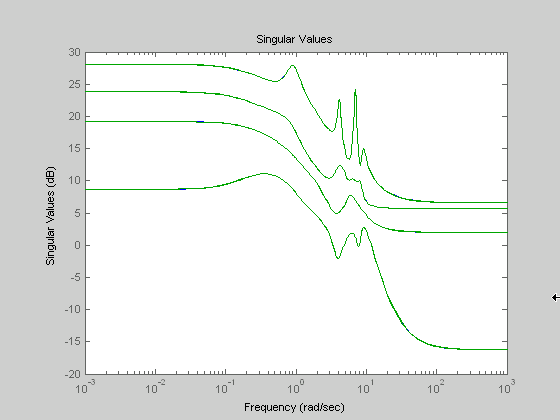
Singular Value Bode Plot of G (30-state, 5 outputs, 4 inputs) shows a singular value Bode plot of a random system G with 20 states, 5 output and 4 inputs. The error system between G and its Zeroth order Hankel MDA has it infinity norm equals to an all pass function, as shown in All-Pass Error System Between G and Zeroth Order G Anticausal.

The Zeroth order Hankel MDA and its error system sigma plot are obtained via commands

[g0,redinfo0] = hankelmr(G,0);
sigma(G-redinfo0.Ganticausal)

This interesting all-pass property is unique in Hankel MDA model reduction.

Singular Value Bode Plot of G (30-state, 5 outputs, 4 inputs)

All-Pass Error System Between G and Zeroth Order G Anticausal

Algorithms

Given a state-space (A,B,C,D) of a system and k, the desired reduced order, the following steps will produce a similarity transformation to truncate the original state-space system to the k^th order reduced model.

Find the controllability and observability Gramians P and Q.
Form the descriptor
$E = Q P - ρ^{2} I$
where $σ_{k} > ρ \geq σ_{k + 1}$ , and descriptor state-space
Take SVD of descriptor E and partition the result into k^th order truncation form
$\begin{array}{l} [\begin{matrix} E s - \bar{A} & \bar{B} \\ \bar{C} & \bar{D} \end{matrix}] = [\begin{matrix} ρ^{2} A^{T} + Q A P & Q B \\ C P & D \end{matrix}] \\ E = [U_{E 1}, U_{E 2}] [\begin{matrix} Σ_{E} 0 & 0 \\ 0 & 0 \end{matrix}] [\begin{matrix} V_{E 1}^{T} \\ V_{E 2}^{T} \end{matrix}] \end{array}$
Apply the transformation to the descriptor state-space system above we have
$\begin{array}{l} [\begin{matrix} A_{11} & A_{12} \\ A_{21} & A_{22} \end{matrix}] = [\begin{matrix} U_{E 1}^{T} \\ U_{E 2}^{T} \end{matrix}] (ρ^{2} A^{T} + Q A P) [\begin{matrix} V_{E 1} & V_{E 2} \end{matrix}] \\ [\begin{matrix} B_{1} \\ B_{2} \end{matrix}] = [\begin{matrix} U_{E 1}^{T} \\ U_{E 2}^{T} \end{matrix}] [\begin{matrix} Q B & - C^{T} \end{matrix}] \\ [\begin{matrix} C_{1} & C_{2} \end{matrix}] = [\begin{matrix} C P \\ - ρ B^{T} \end{matrix}] [\begin{matrix} V_{E 1} & V_{E 2} \end{matrix}] \\ D_{1} = D \end{array}$
Form the equivalent state-space model.
$[\begin{matrix} \tilde{A} & \tilde{B} \\ \tilde{C} & \tilde{D} \end{matrix}] = [\begin{matrix} \sum_{E}^{- 1} (A_{11} - A_{12} A_{22}^{†} A_{21}) & \sum_{E}^{- 1} (B_{1} - A_{12} A_{22}^{†} B_{2}) \\ C_{1} - C_{2} A_{22}^{†} A_{21} & D_{1} - C_{2} A_{22}^{†} B_{2} \end{matrix}]$
The final k^th order Hankel MDA is the stable part of the above state-space realization. Its anticausal part is stored in redinfo.Ganticausal.

The proof of the Hankel MDA algorithm can be found in [2]. The error system between the original system G and the Zeroth Order Hankel MDA G₀ is an all-pass function [1].

References

[1] Glover, K., “All Optimal Hankel Norm Approximation of Linear Multivariable Systems, and Their L_∝-error Bounds,” Int. J. Control, vol. 39, no. 6, pp. 1145-1193, 1984.

[2] Safonov, M.G., R.Y. Chiang, and D.J.N. Limebeer, “Optimal Hankel Model Reduction for Nonminimal Systems,” IEEE Trans. on Automat. Contr., vol. 35, no. 4, April 1990, pp. 496-502.

Version History

Introduced before R2006a