Main Content

mussv

Compute bounds on structured singular value (µ)

Description

bounds = mussv(M,BlockStructure) calculates upper and lower bounds on the structured singular value, or µ, of the system described by M and a given block-diagonal uncertainty Delta configured as follows.
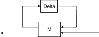
BlockStructure is a matrix encoding the block-diagonal structure of Delta. μ is a generalization of the singular value for uncertain systems. M is a numeric array, a state-space (ss) model, or a frequency response (frd) model.

In practice, μ is difficult to compute exactly, so the software instead computes lower and upper bounds, μ¯ and μ¯, returned in bounds. The upper bound μ¯ can be used as a measure of the system's robust performance. (See Robust Performance Measure for Mu Synthesis.)

example

[bounds,muinfo] = mussv(M,BlockStructure) returns a structure containing more detailed information. To extract the information in muinfo, use mussvextract.

[bounds,muinfo] = mussv(M,BlockStructure,opt) specifies additional computation options.

Examples

collapse all

Compute bounds on the structured singular value of a system with three states, three outputs, and three inputs, with respect to an uncertain structure consisting of one instance of a diagonal real uncertainty and two repetitions of another diagonal real uncertainty. Start with a state-space model. For this example use a model with random dynamics.

rng('default');   % for repeatability
Mss = rss(3,3,3);
size(Mss)
State-space model with 3 outputs, 3 inputs, and 3 states.

Compute frequency response data for Mss over a range of frequencies.

w = logspace(-5,5,100);
Mfr = freqresp(Mss,w);
size(Mfr)
ans = 1×3

     3     3   100

Create a matrix representing the uncertainty structure. To indicate the diagonal scalar uncertainty, set the first row to [-1,0]. To indicate the repeating instances of the second real uncertainty, set the second row to [-2,0].

BlockStructure = [-1,0;-2,0];

Compute the structured singular value. The 's' option suppresses the progress display during computation.

[bounds,muinfo] = mussv(Mfr,BlockStructure,'s');
size(bounds)
ans = 1×3

     1     2   100

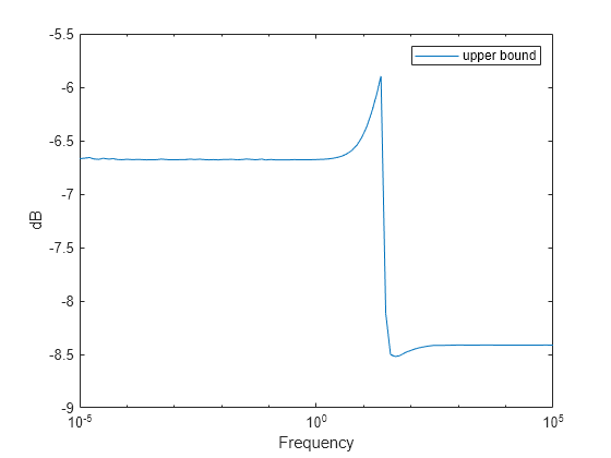
Each row of bounds contains the upper and lower bound on the structured singular value at a frequency in w. Examine the upper bound as a function of frequency.

upper = mag2db(squeeze(bounds(1,1,:)));
semilogx(w,upper);
legend("upper bound")
xlabel("Frequency")
ylabel("dB")

Figure contains an axes object. The axes object with xlabel Frequency, ylabel dB contains an object of type line. This object represents upper bound.

Input Arguments

collapse all

Input matrix, specified as a numeric array of frequency response data, an frd model, or an ss model.

If M is an N-dimensional numeric array with N ≥ 3, then the computation is performed pointwise along the third and higher array dimensions.

If M is a frd object, the computations are performed pointwise in frequency (as well as any array dimensions).

Uncertainty block structure, specified as a two-column matrix that encodes the block-diagonal structure of the uncertainty. BlockStructure has as many rows as there are uncertainty blocks in the perturbation structure. The i-th row of BlockStructure defines the dimensions of the i-th perturbation block as follows:

  • If BlockStructure(i,:) = [-r 0], then the i-th block is an r-by-r repeated, diagonal real scalar perturbation.

  • if BlockStructure(i,:) = [r 0], then the i-th block is an r-by-r repeated, diagonal complex scalar perturbation;

  • if BlockStructure(i,:) = [r c], then the i-th block is an r-by-c complex full-block perturbation.

If you omit BlockStructure, then mussv uses the default ones(size(M,1),2), which specifies a perturbation structure of all 1-by-1 complex blocks. For this usage, size(M,1) must not equal size(M,2).

Alternatively, can also specify uncertainty structure using the BlockStructure output argument of lftdata.

Computation options, specified as a character vector, containing any combination of the following characters.

Option

Meaning

'a'

Compute upper bound to greatest accuracy, using LMI solver.

'an'

Same as 'a', but without automatic prescaling.

'd'

Display warnings.

'f'

Fast upper bound (typically not as tight as the default 'a').

'gN'

Use gain-based lower bound method multiple times. The value of N sets the number of times, according to 10+N*10. For example, 'g6' uses gain-based lower bound 70 times. Larger numbers typically give better lower bounds.

If all uncertainty blocks described by blk are real, then the default is 'g1'. If at least one uncertainty block is complex, then mussv uses power iteration lower bound by default.

'p'

Use power iteration method to compute lower bound. When at least one of the uncertainty blocks described by blk is complex, then 'p' is the default lower bound method.

'i'

Reinitialize lower bound computation at each new matrix (only relevant if M is an N-dimensional array or frd).

'mN'

Randomly reinitialize lower bound iteration multiple times. N is an integer between 1 and 9. For example, 'm7' randomly reinitializes the lower bound iteration 7 times. Larger numbers typically give better lower bounds.

'o'

Run “old” algorithms, from version 3.1.1 and before. Included to allow exact replication of earlier calculations.

's'

Suppress progress information (silent).

'U'

Upper-bound “only” (lower bound uses a fast/cheap algorithm).

'x'

Decrease iterations in lower bound computation (faster but not as tight as default). Use 'U' for an even faster lower bound.

Example: 'Ufs' computes the upper bound only, using a fast algorithm, and suppresses the progress display during computation.

Output Arguments

collapse all

Bounds on structured singular value, returned as an array. If M is:

  • A two-dimensional matrix or a state-space model, then bounds is a two-element array of the form [ub lb], where ub is the upper bound and lb is the lower bound. In this case, for all values of Delta with block-diagonal structure defined by BlockStructure and with norm less than 1/ub, the matrix I - M*Delta is not singular. Moreover, there is a matrix DeltaS with the same structure and norm equal to 1/lb, for which the matrix I - M*DeltaS is singular.

  • An N-dimensional array, then mussv computes the upper and lower bounds pointwise along the third and higher array dimensions. For example, suppose that M is r-by-c-by-d1-by-...-by-dF. Then bounds is 1-by-2-by-d1-by-...-by-dF. In single-index notation, bounds(1,1,i) is the upper bound for the structured singular value of M(:,:,i), and bounds(1,2,i) is the lower bound for the structured singular value of M(:,:,i). Here, any i between 1 and d1·d2...dF (the product of the dk) is valid.

  • An frd model with N frequency points, then mussv computes the upper and lower bounds pointwise along in frequency for frd models. In this case, bounds is a 1-by-2-by-N array, consisting of N rows, each of the form [ub lb]. Each row contains the upper and lower bounds for the structured singular value at the corresponding frequency.

Additional information about the structured singular value bounds, returned as a structure. To interpret the data in this structure, use mussvextract.

Algorithms

mussv computes the lower bound using a power method of [7] and [4], and the upper bound using the balanced/AMI technique of [6] for computing the upper bound from [2]. In the upper bound computation, the matrix is first balanced using either a variation of Osborne's method ([3]) generalized to handle repeated scalar and full blocks, or a Perron approach. This computation generates the standard upper bound for the associated complex µ problem. The Perron eigenvector method is based on an idea of Safonov ([5]). It gives the exact computation of µ for positive matrices with scalar blocks, but is comparable to Osborne on general matrices. Both the Perron and Osborne methods have been modified to handle repeated scalar and full blocks. Perron is faster for small matrices but has a growth rate of n3, compared with less than n2 for Osborne. This is partly due to the MATLAB® implementation, which greatly favors Perron. The default is to use Perron for simple block structures and Osborne for more complicated block structures. A sequence of improvements to the upper bound is then made based on various equivalent forms of the upper bound. A number of descent techniques are used that exploit the structure of the problem, concluding with general purpose LMI optimization ([1]) to obtain the final answer.

Peter Young and Matt Newlin wrote the original version of mussv.

References

[1] Boyd, S. and L. El Ghaoui, “Methods of centers for minimizing generalized eigenvalues,” Linear Algebra and Its Applications, Vol. 188–189, 1993, pp. 63–111.

[2] Fan, M., A. Tits, and J. Doyle, “Robustness in the presence of mixed parametric uncertainty and unmodeled dynamics,” IEEE Transactions on Automatic Control, Vol. AC–36, 1991, pp. 25–38.

[3] Osborne, E., “On preconditioning of matrices,” Journal of Associated Computer Machines, Vol. 7, 1960, pp. 338–345.

[4] Packard, A.K., M. Fan and J. Doyle, “A power method for the structured singular value,” Proc. of 1988 IEEE Conference on Control and Decision, December 1988, pp. 2132–2137.

[5] Safonov, M., “Stability margins for diagonally perturbed multivariable feedback systems,” IEEE Proc., Vol. 129, Part D, 1992, pp. 251–256.

[6] Young, P. and J. Doyle, “Computation of with real and complex uncertainties,” Proceedings of the 29th IEEE Conference on Decision and Control, 1990, pp. 1230–1235.

[7] Young, P., M. Newlin, and J. Doyle, “Practical computation of the mixed problem,” Proceedings of the American Control Conference, 1992, pp. 2190–2194.

Version History

Introduced before R2006a