Calculate Latency and Doppler in a Satellite Scenario
This example shows how to model a GPS satellite constellation from a SEM almanac, analyze access between the satellites and a ground station, and calculate the latency and the Doppler shift between the satellites and the ground station.
Create a Satellite Scenario
Create a satellite scenario with a start time of 11-January-2020 2:50:00 PM UTC and a stop time 3 days later. Set the simulation sample time to 60 seconds.
startTime = datetime(2020,1,11,14,50,0);
stopTime = startTime + days(3);
sampleTime = 60;                         % In seconds
sc = satelliteScenario( ...
    startTime,stopTime,sampleTime);
Add a Satellite to the Scenario
Add a satellite to the scenario from the gpsAlmanac.txt SEM almanac file. To obtain the latest SEM almanac file, visit the Navigation Center website at www.navcen.uscg.gov and search for 'SEM Almanac'.
sat = satellite(sc,"gpsAlmanac.txt");The default orbit propagator when creating satellites using SEM almanac is gps. This can be verified by observing the OrbitPropagator property. Additionally, the output of the orbitalElements function contains GPS satellite-specific information.
orbitProp = sat(1).OrbitPropagator
orbitProp =
"gps"
elements = orbitalElements(sat(1))
elements = struct with fields:
                                  PRN: 1
                        GPSWeekNumber: 2087
               GPSTimeOfApplicability: 589824
                      SatelliteHealth: 0
                        SemiMajorAxis: 2.6560e+07
                         Eccentricity: 0.0093
                          Inclination: 56.0665
    GeographicLongitudeOfOrbitalPlane: -40.4778
                 RateOfRightAscension: -4.6166e-07
                    ArgumentOfPerigee: 43.3831
                          MeanAnomaly: 172.6437
                               Period: 4.3077e+04
Add a Ground Station
Add the Madrid Deep Space Communications Complex as the ground station of interest, and specify its latitude and longitude.
name = "Madrid Deep Space Communications Complex";
lat = 40.43139;                                    % In degrees
lon = -4.24806;                                    % In degrees
gs = groundStation(sc, ...
    Name=name,Latitude=lat,Longitude=lon);
Add an Access Analysis and Visualize Scenario
Add access analysis between the GPS satellites and Madrid ground station, which determines when the ground station is visible to the satellites. This helps in visualizing which satellites are visible to the ground station with time.
ac = access(sat,gs);
Visualize the scenario by launching a satellite scenario viewer. Set ShowDetails of the viewer to false to ensure the visualization is not cluttered. Set the camera position to bring all satellites that have access to the ground station into view.
v = satelliteScenarioViewer(sc,ShowDetails=false);
campos(v, ...
    29, ...                                        % Latitude in degrees
    -19, ...                                       % Longitude in degrees
    7.3e7);                                        % Altitude in meters

Calculate Latency and Rate of Change of Latency
Calculate the propagation delay from the GPS satellites to the Madrid ground station using the latency function. Also, compute the rate of change of propagation delay.
% Calculate propagation delay from each satellite to the ground station.
% The latency function internally performs access analysis and returns NaN
% whenever there is no access.
[delay,time] = latency(sat,gs);
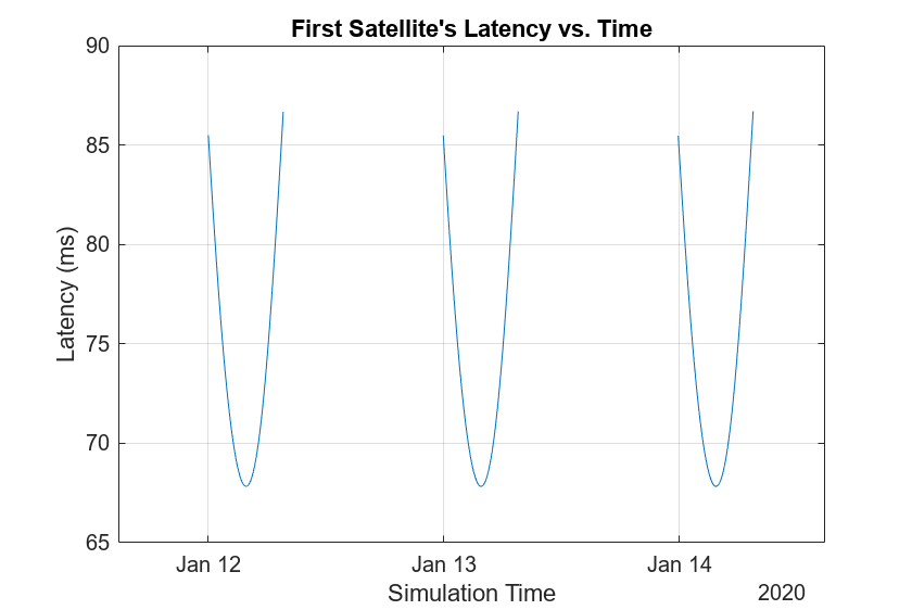
Plot the propagation delay corresponding to the first satellite. You may choose to plot the propagation delay corresponding to all satellites. However, this example plots it only for the first satellite to serve as a demonstration and to reduce plot clutter.
plot(time,delay(1,:)*1000)                  % Plot in milliseconds
xlim([time(1) time(end)])
title("First Satellite's Latency vs. Time")
xlabel("Simulation Time")
ylabel("Latency (ms)")
grid on

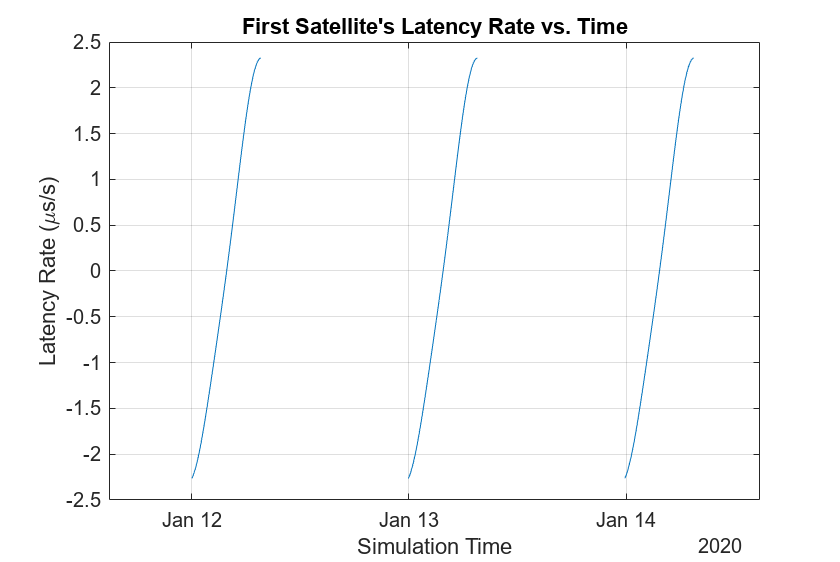
Plot the rate of change of propagation delay corresponding to the first satellite.
latencyRate = diff(delay,1,2)/sampleTime;
plot(time(1:end-1),latencyRate(1,:)*1e6)          % Plot in microseconds/second
xlim([time(1) time(end-1)])
title("First Satellite's Latency Rate vs. Time")
xlabel("Simulation Time")
ylabel("Latency Rate (\mus/s)")
grid on

Calculate Doppler Shift and Rate of Change of Doppler Shift
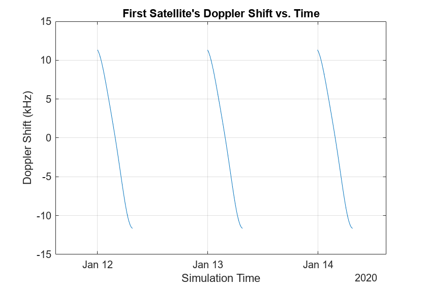
This example considers a C band frequency of 5 GHz. Calculate the Doppler shift and the variation of Doppler shift using the dopplershift function.
% Emitted carrier frequency in Hz
fc = 5e9;
% Calculate Doppler shift and get additional information about Doppler. The
% Doppler information output contains relative velocity and Doppler rate.
% The dopplershift function internally performs access analysis and returns
% NaN whenever there is no access.
[fShift,time,dopplerInfo] = dopplershift(sat,gs,Frequency=fc);
Plot the Doppler shift corresponding to the first satellite.
plot(time,fShift(1,:)/1e3)                        % Plot in kHz
xlim([time(1) time(end)])
title("First Satellite's Doppler Shift vs. Time")
xlabel("Simulation Time")
ylabel("Doppler Shift (kHz)")
grid on

Plot the Doppler rate corresponding to the first satellite.
plot(time(1:end-1),dopplerInfo.DopplerRate(1,:))  % Plot in Hz/s
xlim([time(1) time(end-1)])
title("First Satellite's Doppler Rate vs. Time")
xlabel("Simulation Time")
ylabel("Doppler Rate (Hz/s)")
grid on

Show the name and orbit of the first satellite and plot its future ground track, or lead time, over 12 hours. Dashed yellow shows the future ground track, and solid yellow shows the past ground track.
sat(1).ShowLabel = true;
show(sat(1).Orbit);
groundTrack(sat(1), ...
    LeadTime=12*3600);   % In seconds
campos(v,84,-176,7.3e7);

Play the scenario with the satellites and ground station.
play(sc)

See Also
Objects
Functions
orbitalElements|aer|play