tsa

Compute the time-synchronous average of a noisy sinusoid.

Generate a signal consisting of a sinusoid embedded in white Gaussian noise. The signal is sampled at 500 Hz for 20 seconds. Specify a sinusoid frequency of 10 Hz and a noise variance of 0.01. Plot one period of the signal.

fs = 500;
t = 0:1/fs:20-1/fs;

f0 = 10;
y = sin(2*pi*f0*t) + randn(size(t))/10;

plot(t,y)
xlim([0 1/f0])

Compute the time-synchronous average of the signal. For the synchronizing signal, use a set of pulses with the same period as the sinusoid. Use tsa without output arguments to display the result.

tPulse = 0:1/f0:max(t);

tsa(y,fs,tPulse)

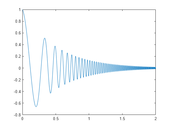
Generate a signal that consists of an exponentially damped quadratic chirp. The signal is sampled at 1 kHz for 2 seconds. The chirp has an initial frequency of 2 Hz that increases to 28 Hz after the first second. The damping has a characteristic time of 1/2 second. Plot the signal.

fs = 1e3;
t = 0:1/fs:2;

x = exp(-2*t').*chirp(t',2,1,28,'quadratic');

plot(t,x)

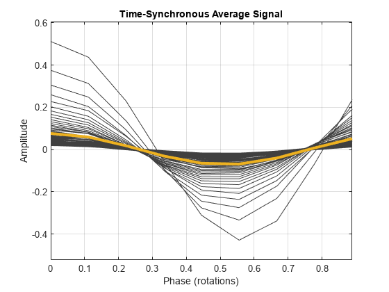
Create a duration array using the time vector. Construct a timetable with the duration array and the signal. Determine the pulse times using the locations of the signal peaks. Display the time-synchronous average.

ts = seconds(t)';
tx = timetable(ts,x);

[~,lc] = findpeaks(x,t);
tsa(tx,lc)

Compute the time-synchronous average. View the types of the output arguments. The sample times are stored in a duration array.

[xta,xt,xp,xrpm] = tsa(tx,lc);
whos x*

  Name         Size            Bytes  Class        Attributes

  x         2001x1             16008  double                 
  xp           9x1              1133  timetable              
  xrpm         1x1                 8  double                 
  xt           9x1                74  duration               
  xta          9x1              1129  timetable              

Convert the duration array to a datetime vector. Construct a timetable using the datetime vector and the signal. Compute the time-synchronous average, but now average over sets of 15 rotations.

View the types of the output arguments. The sample times are again stored in a duration array, even though the input timetable used a datetime vector.

dtb = datetime(datevec(ts));
dtt = timetable(dtb,x);

nr = 15;
tsa(dtt,lc,'NumRotations',nr)

[dta,dt,dp,drpm] = tsa(dtt,lc,'NumRotations',nr);
whos d*

  Name         Size            Bytes  Class        Attributes

  dp         135x1              3149  timetable              
  drpm         1x1                 8  double                 
  dt         135x1              1082  duration               
  dta        135x1              3145  timetable              
  dtb       2001x1             32016  datetime               
  dtt       2001x1             49001  timetable              

Compute the time-synchronous average of the position of a fan blade as it slows down after switchoff.

A desk fan spinning at 2400 rpm is turned off. Air resistance (with a negligible contribution from bearing friction) causes the fan rotor to stop in approximately 5 seconds. A high-speed camera measures the x-coordinate of one of the fan blades at a rate of 1 kHz.

fs = 1000;
t = 0:1/fs:5-1/fs;

rpm0 = 2400;

Idealize the fan blade as a point mass circling the rotor center at a radius of 10 cm. The blade experiences a drag force proportional to speed, resulting in the following expression for the phase angle:

where ${\mathit{f}}_0$ is the initial frequency and $\mathit{T}=0.75$ second is the decay time.

a = 0.1;
f0 = rpm0/60;
T = 0.75;

phi = 2*pi*f0*T*(1-exp(-t/T));

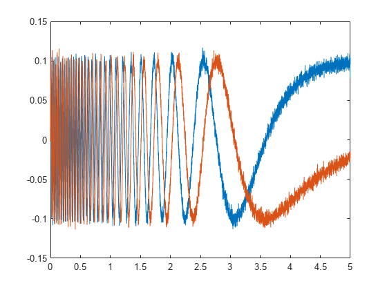
Compute and plot the x- and y-coordinates. Add white Gaussian noise.

x = a*cos(phi) + randn(size(phi))/200;
y = a*sin(phi) + randn(size(phi))/200;

plot(t,x,t,y)

Determine the synchronizing signal. Use the tachorpm function to find the pulse times. Limit the search to times before 2.5 seconds. Plot the rotational speed to see its exponential decay.

[rpm,~,tp] = tachorpm(x(t<2.5),fs);
tachorpm(x(t<2.5),fs)

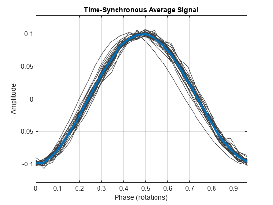
Compute and plot the time-synchronous average signal, which corresponds to a period of a sinusoid. Perform the averaging in the frequency domain.

clf
tsa(x,fs,tp,Method="fft")